Home · Book Reports · 2018 · Basics of Linear Algebra for Machine Learning - Discover the Mathematical Language of Data in Python

designates my notes. / designates important.

Thoughts

Overall I’d say it is far too simple, but would be a great to whet your appetite if you didn’t know anything.

The pace eventually picks up into an extremely enjoyable read, although still too simple. It is, nevertheless, straight to the point and not proof heavy.

It would certainly make a good introduction if you want to go farther, but does offer enough to let you start using machine learning with more understanding (although not a deep understanding, which might not be necessary).

It includes lots of clear code examples for very basic calculations, but no mention of any actual applications.

It does have a lot of repetition at the beginning and end of each chapter; restating goals. It could probably have been done in 150 pages instead of 200. The links are mostly to wikipedia articles and the links to books on amazon are redundant; the same half dozen books are linked over and over. Still, easy enough to glide past them.

Books

• I’d also recommend a good textbook on multivariate statistics, which is the intersection of linear algebra, and numerical statistical methods. Some good introductory textbooks include:

• Applied Multivariate Statistical Analysis, Richard Johnson and Dean Wichern,

• Applied Multivariate Statistical Analysis, Wolfgang Karl Hardle and Leopold Simar, 2015.

• There are also many good free online books written by academics. See the end of the Linear Algebra page on Wikipedia for an extensive (and impressive) reading list.

• Linear Algebra at MIT by Gilbert Strang. https://ocw.mit.edu/courses/mathematics/18-06-linear-algebra-spring-2010/index. htm

• The Matrix in Computer Science at Brown by Philip Klein. http://cs.brown.edu/courses/cs053/current/index.htm

• Computational Linear Algebra for Coders at University of San Francisco by Rachel Thomas. https://github.com/fastai/numerical-linear-algebra/

• The Language and Grammar of Mathematics, Timothy Gowers. http://assets.press.princeton.edu/chapters/gowers/gowers_I_2.pdf

Table of Contents

Part 1: Introduction

• Welcome

Part 2: Foundations

• 01: Introduction to Linear Algebra
• 02: Linear Algebra and Machine Learning
• 03: Examples of Linear Algebra in Machine Learning

Part 3: Numpy

• 04: Introduction to NumPy Arrays
• 05: Index, Slice and Reshape NumPy Arrays
• 06: NumPy Array Broadcasting

Part 4: Matrices

• 07: Vectors and Vector Arithmetic
• 08: Vector Norms
• 09: Matrices and Matrix Arithmetic
• 10: Types of Matrices
• 11: Matrix Operations
• 12: Sparse Matrices
• 13: Tensors and Tensor Arithmetic

Part 5: Factorization

• 14: Matrix Decompositions
• 15: Eigendecomposition
• 16: Singular Value Decomposition

Part 6: Statistics

• 17: Introduction to Multivariate Statistics
• 18: Principal Component Analysis
• 19: Linear Regression
• Appendix

• Actual pages numbers.

Part 1: Introduction

· 01: Introduction to Linear Algebra

Part 2: Foundations

· 02: Linear Algebra and Machine Learning

· 03: Examples of Linear Algebra in Machine Learning

page 14:

• L2 and L1 forms of regularization. Both of these forms of regularization are in fact a measure of the magnitude or length of the coefficients as a vector and are methods lifted directly from linear algebra called the vector norm.

Part 3: Numpy

· 04: Introduction to NumPy Arrays

· 05: Index, Slice and Reshape NumPy Arrays

· 06: NumPy Array Broadcasting

page 36:

• Broadcasting is the name given to the method that NumPy uses to allow array arithmetic between arrays with a different shape or size. Although the technique was developed for NumPy, it has also been adopted more broadly in other numerical computational libraries, such as Theano, TensorFlow, and Octave.

• In the context of deep learning, we also use some less conventional notation. We allow the addition of matrix and a vector, yielding another matrix: C = A + b, where C_i,j = A_i,j + b_j . In other words, the vector b is added to each row of the matrix. This shorthand eliminates the need to define a matrix with b copied into each row before doing the addition. This implicit copying of b to many locations is called broadcasting. — Page 34, Deep Learning, 2016.

page 40:

• NumPy will in effect pad missing dimensions with a size of 1 when comparing arrays. Therefore, the comparison between a two-dimensional array A with 2 rows and 3 columns and a vector b with 3 elements:

A.shape = (2 x 3)
b.shape = (3)

• In effect, this becomes a comparison between:

A.shape = (2 x 3)
b.shape = (1 x 3)

• This same notion applies to the comparison between a scalar that is treated as an array with the required number of dimensions:

A.shape = (2 x 3)
b.shape = (1)

• This becomes a comparison between:

A.shape = (2 x 3)
b.shape = (1 x 1)

• When the comparison fails, the broadcast cannot be performed, and an error is raised. The example below attempts to broadcast a two-element array to a 2 × 3 array. This comparison is in effect:

A.shape = (2 x 3)
b.shape = (1 x 2)

• We can see that the last dimensions (columns) do not match and we would expect the broadcast to fail. The example below demonstrates this in NumPy.

Part 4: Matrices

· 07: Vectors and Vector Arithmetic

· 08: Vector Norms

page 53:

• The L1 norm that is calculated as the sum of the absolute values of the vector.

• The L2 norm that is calculated as the square root of the sum of the squared vector values.

• The max norm that is calculated as the maximum vector values.

• The length of a vector is a nonnegative number that describes the extent of the vector in space, and is sometimes referred to as the vector’s magnitude or the norm. — Page 112, No Bullshit Guide To Linear Algebra, 2017.

page 54:

• The length of a vector can be calculated using the L1 norm, where the 1 is a superscript of the L. The notation for the L1 norm of a vector is ||v||_1, where 1 is a subscript. As such, this length is sometimes called the taxicab norm or the Manhattan norm.

L1(v) = ||v||_1  (8.1)

• The L1 norm is calculated as the sum of the absolute vector values, where the absolute value of a scalar uses the notation |a1|. In effect, the norm is a calculation of the Manhattan distance from the origin of the vector space.

||v||_1 = |a_1| + |a_2| + |a_3|  (8.2)

• In several machine learning applications, it is important to discriminate between elements that are exactly zero and elements that are small but nonzero. In these cases, we turn to a function that grows at the same rate in all locations, but retains mathematical simplicity: the L1 norm. — Pages 39-40, Deep Learning, 2016.

• The L1 norm of a vector can be calculated in NumPy using the norm() function with a parameter to specify the norm order,

>>> # vector L1 norm
>>> from numpy import array
>>> from numpy.linalg import norm
>>> # define vector
>>> a = array([1, 2, 3])
>>> print(a)
[1 2 3]
>>> # calculate norm
>>> l1 = norm(a, 1)
>>> print(l1)
6.0

page 55:

• The L2 norm calculates the distance of the vector coordinate from the origin of the vector space. As such, it is also known as the Euclidean norm as it is calculated as the Euclidean distance from the origin.

>>> # vector L2 norm
>>> from numpy import array
>>> from numpy.linalg import norm
>>> # define vector
>>> a = array([1, 2, 3])
>>> print(a)
[1 2 3]
>>> # calculate norm
>>> l2 = norm(a) #default param for L2
>>> print(l2)
3.74165738677

• By far, the L2 norm is more commonly used than other vector norms in machine learning.

page 56:

• The length of a vector can be calculated using the maximum norm, also called max norm. Max norm of a vector is referred to as L^inf where inf is a superscript and can be represented with the infinity symbol. The notation for max norm is ||v||_inf , where inf is a subscript.

L^inf (v) = ||v||_inf  (8.5)

• The max norm is calculated as returning the maximum value of the vector, hence the name.

||v||_inf = max a1, a2, a3  (8.6)

• The max norm of a vector can be calculated in NumPy using the norm() function with the order parameter set to inf.

>>> # vector max norm
>>> from math import inf
>>> from numpy import array
>>> from numpy.linalg import norm
>>> # define vector
>>> a = array([1, 2, 3])
>>> print(a)
[1 2 3]
>>> # calculate norm
>>> maxnorm = norm(a, inf)
>>> print(maxnorm)
3.0

· 09: Matrices and Matrix Arithmetic

page 62:

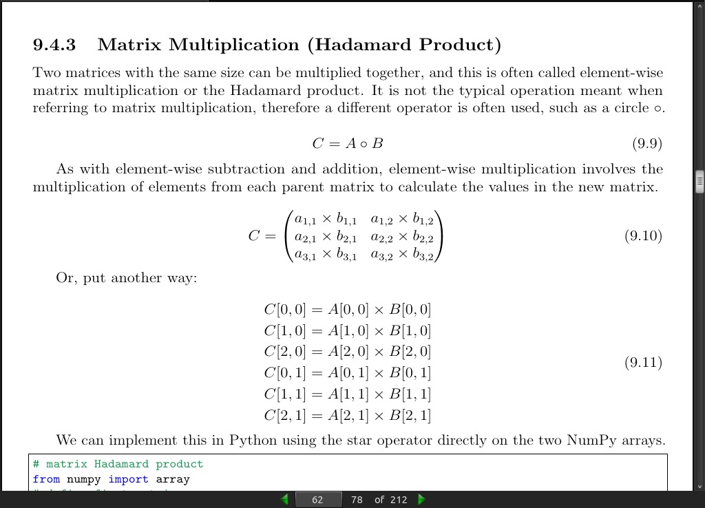
• Two matrices with the same size can be multiplied together, and this is often called element-wise matrix multiplication or the Hadamard product. It is not the typical operation meant when referring to matrix multiplication, therefore a different operator is often used, such as a circle ‘o’.

page 64:

• Dot product

• For example, matrix A has the dimensions m rows and n columns and matrix B has the dimensions n and k. The n columns in A and n rows in B are equal. The result is a new matrix with m rows and k columns.

C(m, k) = A(m, n) · B(n, k)

page 66:

• [Numpy] calculates their dot product using the dot() function and the @ operator.

· 10: Types of Matrices

page 72:

• A symmetric matrix is always square and equal to its own transpose.

page 73:

• A triangular matrix is a type of square matrix that has all values in the upper-right or lower-left of the matrix with the remaining elements filled with zero values.

• NumPy provides functions to calculate a triangular matrix from an existing square matrix. The tril() function to calculate the lower triangular matrix from a given matrix and the triu() to calculate the upper triangular matrix from a given matrix

page 74:

• A diagonal matrix is one where values outside of the main diagonal have a zero value, where the main diagonal is taken from the top left of the matrix to the bottom right.

• A diagonal matrix does not have to be square. In the case of a rectangular matrix, the diagonal would cover the dimension with the smallest length

page 75:

• An identity matrix is a square matrix that does not change a vector when multiplied. The values of an identity matrix are known. All of the scalar values along the main diagonal (top-left to bottom-right) have the value one, while all other values are zero.

• An identity matrix is often represented using the notation I or with the dimensionality I_n , where n is a subscript that indicates the dimensionality of the square identity matrix. In some notations, the identity may be referred to as the unit matrix, or U.

page 76:

• Two vectors are orthogonal when their dot product equals zero.

• An Orthogonal matrix is often denoted as uppercase Q.

page 77:

• A matrix is orthogonal if its transpose is equal to its inverse.

• Another equivalence for an orthogonal matrix is if the dot product of the matrix and itself equals the identity matrix.

Q · Q^T = I

page 78:

-Orthogonal matrices are useful tools as they are computationally cheap and stable to calculate their inverse as simply their transpose.

· 11: Matrix Operations

page 82:

• A square matrix that is not invertible is referred to as singular.

page 83:

• A trace of a square matrix is the sum of the values on the main diagonal of the matrix (top-left to bottom-right).

page 84:

• The determinant describes the relative geometry of the vectors that make up the rows of the matrix. More specifically, the determinant of a matrix A tells you the volume of a box with sides given by rows of A. — Page 119, No Bullshit Guide To Linear Algebra, 2017.

• The intuition for the determinant is that it describes the way a matrix will scale another matrix when they are multiplied together. For example, a determinant of 1 preserves the space of the other matrix. A determinant of 0 indicates that the matrix cannot be inverted.

page 85:

• The rank of a matrix is the estimate of the number of linearly independent rows or columns in a matrix.

• An intuition for rank is to consider it the number of dimensions spanned by all of the vectors within a matrix. For example, a rank of 0 suggest all vectors span a point, a rank of 1 suggests all vectors span a line, a rank of 2 suggests all vectors span a two-dimensional plane.

· 12: Sparse Matrices

page 90:

• It is computationally expensive to represent and work with sparse matrices as though they are dense, and much improvement in performance can be achieved by using representations and operations that specifically handle the matrix sparsity.

page 91:

sparsity = count of zero elements / total elements

page 93:

• Compressed Sparse Row. (CSR) The sparse matrix is represented using three one-dimensional arrays for the non-zero values, the extents of the rows, and the column indexes.

• Compressed Sparse Column. The same as the Compressed Sparse Row method except the column indices are compressed and read first before the row indices.

page 94:

• A dense matrix stored in a NumPy array can be converted into a sparse matrix using the CSR representation by calling the [scipy.sparse] csr matrix() function.

>>> # sparse matrix
>>> from numpy import array
>>> from scipy.sparse import csr_matrix
>>> # create dense matrix
>>> A = array([
[1, 0, 0, 1, 0, 0],
[0, 0, 2, 0, 0, 1],
[0, 0, 0, 2, 0, 0]])

>>> print(A)
[[1 0 0 1 0 0]
[0 0 2 0 0 1]
[0 0 0 2 0 0]]

>>> # convert to sparse matrix (CSR method)
>>> S = csr_matrix(A)
>>> print(S)
>>> (0, 0) 1
>>> (0, 3) 1
>>> (1, 2) 2
>>> (1, 5) 1
>>> (2, 3) 2
>>> 
>>> # reconstruct dense matrix
>>> B = S.todense()
>>> print(B)
[[1 0 0 1 0 0]
[0 0 2 0 0 1]
[0 0 0 2 0 0]]

page 95:

• NumPy does not provide a function to calculate the sparsity of a matrix. Nevertheless, we can calculate it easily by first finding the density of the matrix and subtracting it from one. The number of non-zero elements in a NumPy array can be given by the count nonzero() function and the total number of elements in the array can be given by the size property of the array. Array sparsity can therefore be calculated as

sparsity = 1.0 - count_nonzero(A) / A.size

>>> # sparsity calculation
>>> from numpy import array
>>> from numpy import count_nonzero
>>> # create dense matrix
>>> A = array([
>>> [1, 0, 0, 1, 0, 0],
>>> [0, 0, 2, 0, 0, 1],
>>> [0, 0, 0, 2, 0, 0]])
>>> print(A)
[[1 0 0 1 0 0]
[0 0 2 0 0 1]
[0 0 0 2 0 0]]
>>> # calculate sparsity
>>> sparsity = 1.0 - (count_nonzero(A) / A.size)
>>> print(sparsity)
0.7222222222222222

· 13: Tensors and Tensor Arithmetic

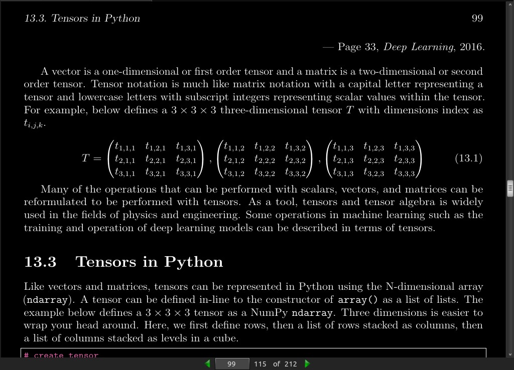
page 099:

page 104:

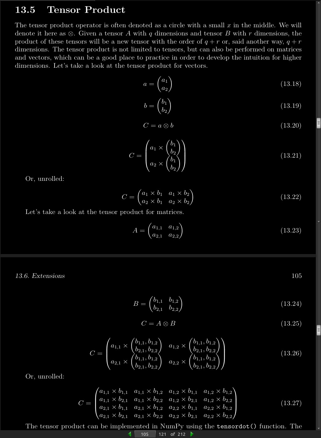
• The tensor product operator is often denoted as a circle with a small x in the middle.

page 105:

• The tensor product can be implemented in NumPy using the tensordot() function.

Part 5: Factorization

· 14: Matrix Decompositions

page 110:

A = LU  (14.2)

• Where A is the square matrix that we wish to decompose, L is the lower triangle matrix and U is the upper triangle matrix.

• The LU decomposition can be implemented in Python with the lu() function.

>>> # LU decomposition
>>> from numpy import array
>>> from scipy.linalg import lu
>>> # define a square matrix
>>> A = array([
>>> [1, 2, 3],
>>> [4, 5, 6],
>>> [7, 8, 9]])
>>> print(A)
[[1 2 3]
[4 5 6]
[7 8 9]]


>>> # factorize
>>> P, L, U = lu(A)
>>> print(P)
[[ 0. 1. 0.]
 [ 0. 0. 1.]
 [ 1. 0. 0.]]

>>> print(L)
[[ 1.         0.  0. ]
 [ 0.14285714 1.  0. ]
 [ 0.57142857 0.5 1. ]]

>>> print(U)
[[ 7.00000000e+00 8.00000000e+00  9.00000000e+00]
 [ 0.00000000e+00 8.57142857e-01  1.71428571e+00]
 [ 0.00000000e+00 0.00000000e+00 -1.58603289e-16]]

>>> # reconstruct
>>> B = P.dot(L).dot(U)
>>> print(B)
[[ 1. 2. 3.]
 [ 4. 5. 6.]
 [ 7. 8. 9.]]

page 111:

A = QR  (14.5)

• Where A is the matrix that we wish to decompose, Q a matrix with the size m × m, and R is an upper triangle matrix with the size m × n.

• The QR decomposition can be implemented in NumPy using the qr() function.

page 112:

• By default, the function returns the Q and R matrices with smaller or reduced dimensions that is more economical. We can change this to return the expected sizes of m × m for Q and m × n for R by specifying the mode argument as ‘complete’,

>>> # QR decomposition
>>> from numpy import array
>>> from numpy.linalg import qr
>>> # define rectangular matrix
>>> A = array([
>>> [1, 2],
>>> [3, 4],
>>> [5, 6]])
>>> print(A)
[[1 2]
 [3 4]
 [5 6]]

>>> # factorize
>>> Q, R = qr(A, ✬complete✬)
>>> print(Q)
[[-0.16903085 0.89708523 0.40824829]
[-0.50709255 0.27602622 -0.81649658]
[-0.84515425 -0.34503278 0.40824829]]

>>> print(R)
[[-5.91607978 -7.43735744]
 [ 0.          0.82807867]
 [ 0.          0. ]]

>>> # reconstruct
>>> B = Q.dot(R)
>>> print(B)
[[ 1. 2.]
 [ 3. 4.]
 [ 5. 6.]]

• The Cholesky decomposition is for square symmetric matrices where all values are greater than zero, so-called positive definite matrices.

A = L L^T  (14.7)

page 113:

• L is the lower triangular matrix and L^T is the transpose of L.

• The decompose can also be written as the product of the upper triangular matrix, for example:

A = U^T U  (14.8)

• When decomposing symmetric matrices, the Cholesky decomposition is nearly twice as efficient as the LU decomposition and should be preferred in these cases.

• The Cholesky decomposition can be implemented in NumPy by calling the cholesky() function.

· 15: Eigendecomposition

page 117:

• This is called the eigenvalue equation, where A is the parent square matrix that we are decomposing, v is the eigenvector of the matrix, and λ is the lowercase Greek letter lambda and represents the eigenvalue scalar.

Av = λv

• The parent matrix can be shown to be a product of the eigenvectors and eigenvalues.

A = QΛQT  (15.4)

• Where Q is a matrix comprised of the eigenvectors, Λ is the uppercase Greek letter lambda and is the diagonal matrix comprised of the eigenvalues

• eigen (pronounced eye-gan) is a German word that means own or innate, as in belonging to the parent matrix.

page 118:

• Almost all vectors change direction, when they are multiplied by A. Certain exceptional vectors x are in the same direction as Ax. Those are the “eigenvectors”. Multiply an eigenvector by A, and the vector Ax is the number λ times the original x. […] The eigenvalue λ tells whether the special vector x is stretched or shrunk or reversed or left unchanged — when it is multiplied by A. — Page 289, Introduction to Linear Algebra, Fifth Edition, 2016.

• Eigendecomposition can also be used to calculate the principal components of a matrix in the Principal Component Analysis method or PCA that can be used to reduce the dimensionality of data in machine learning.

• Eigenvectors are unit vectors,

• They are often referred as right vectors, which simply means a column vector (as opposed to a row vector or a left vector).

page 119:

>>> # eigendecomposition
>>> from numpy import array
>>> from numpy.linalg import eig
>>> # define matrix
>>> A = array([
>>> [1, 2, 3],
>>> [4, 5, 6],
>>> [7, 8, 9]])
>>> print(A)
[[1 2 3]
 [4 5 6]
 [7 8 9]]

>>> # factorize
>>> values, vectors = eig(A)
>>> 15.5. Confirm an Eigenvector and Eigenvalue
>>>  119
>>> print(values)
[ 1.61168440e+01 -1.11684397e+00 -9.75918483e-16]

>>> print(vectors)
[[-0.23197069 -0.78583024 0.40824829]
 [-0.52532209 -0.08675134 -0.81649658]
 [-0.8186735 0.61232756 0.40824829]]

>>> # confirm eigenvector
>>> from numpy import array
>>> from numpy.linalg import eig
>>> # define matrix
>>> A = array([
>>> [1, 2, 3],
>>> [4, 5, 6],
>>> [7, 8, 9]])
>>> # factorize
>>> values, vectors = eig(A)
>>> # confirm first eigenvector
>>> B = A.dot(vectors[:, 0])
>>> print(B)
[ -3.73863537 -8.46653421 -13.19443305]

>>> C = vectors[:, 0] * values[0]
>>> print(C)
[ -3.73863537 -8.46653421 -13.19443305]

page 120:

• We can reverse the process and reconstruct the original matrix given only the eigenvectors and eigenvalues. First, the list of eigenvectors must be taken together as a matrix, where each vector becomes a row. The eigenvalues need to be arranged into a diagonal matrix. The NumPy diag() function can be used for this. Next, we need to calculate the inverse of the eigenvector matrix, which we can achieve with the inv() NumPy function. Finally, these elements need to be multiplied together with the dot() function.

>>> # reconstruct matrix
>>> from numpy import diag
>>> from numpy.linalg import inv
>>> from numpy import array
>>> from numpy.linalg import eig
>>> # define matrix
>>> A = array([
>>> [1, 2, 3],
>>> [4, 5, 6],
>>> [7, 8, 9]])
>>> print(A)
[[1 2 3]
 [4 5 6]
 [7 8 9]]

>>> # factorize
>>> values, vectors = eig(A)
>>> # create matrix from eigenvectors
>>> Q = vectors
>>> # create inverse of eigenvectors matrix
>>> R = inv(Q)
>>> # create diagonal matrix from eigenvalues
>>> L = diag(values)
>>> # reconstruct the original matrix
>>> B = Q.dot(L).dot(R)
>>> print(B)
[[ 1. 2. 3.]
 [ 4. 5. 6.]
 [ 7. 8. 9.]]

· 16: Singular Value Decomposition

page 124:

• Where A is the real m x n matrix that we wish to decompose, U is an m × m matrix, Σ represented by the uppercase Greek letter sigma) is an m × n diagonal matrix, and V T is the V transpose of an n × n matrix

A = U Σ V^T  (16.1)

• The diagonal values in the Σ matrix are known as the singular values of the original matrix A. The columns of the U matrix are called the left-singular vectors of A, and the columns of V are called the right-singular vectors of A.

• The SVD can be calculated by calling the svd() function.

page 125:

>>> # singular-value decomposition
>>> from numpy import array
>>> from scipy.linalg import svd
>>> # define a matrix
>>> A = array([
>>> [1, 2],
>>> [3, 4],
>>> [5, 6]])
>>> print(A)
[[1 2]
 [3 4]
 [5 6]]

>>> # factorize
>>> U, s, V = svd(A)
>>> print(U)
[[-0.2298477   0.88346102  0.40824829]
 [-0.52474482  0.24078249 -0.81649658]
 [-0.81964194 -0.40189603  0.40824829]]

>>> print(s)
[ 9.52551809 0.51430058]

>>> print(V)
[[-0.61962948 -0.78489445]
 [-0.78489445  0.61962948]]

• The original matrix can be reconstructed from the U , Σ, and V T elements. The U , s, and V elements returned from the svd() cannot be multiplied directly. The s vector must be converted into a diagonal matrix using the diag() function. By default, this function will create a square matrix that is m × m, relative to our original matrix. This causes a problem as the size of the matrices do not fit the rules of matrix multiplication, where the number of columns in a matrix must match the number of rows in the subsequent matrix. After creating the square Σ diagonal matrix, the sizes of the matrices are relative to the original n × m matrix that we are decomposing, as follows:

U (m × m) · Σ(m × · T (n ×m) V n)  (16.2)

• Where, in fact, we require:

U (m × m) · Σ(m × n) · V T (n × n)  (16.3)

• We can achieve this by creating a new Σ matrix of all zero values that is m × n (e.g. more rows) and populate the first n × n part of the matrix with the square diagonal matrix calculated via diag().

>>> # reconstruct rectangular matrix from svd
>>> from numpy import array
>>> from numpy import diag
>>> from numpy import zeros
>>> from scipy.linalg import svd
>>> # define matrix
>>> A = array([
>>> [1, 2],
>>> [3, 4],
>>> [5, 6]])
>>> print(A)
[[1 2]
 [3 4]
 [5 6]]

>>> # factorize
>>> U, s, V = svd(A)
>>> # create m x n Sigma matrix
>>> Sigma = zeros((A.shape[0], A.shape[1]))
>>> # populate Sigma with n x n diagonal matrix
>>> Sigma[:A.shape[1], :A.shape[1]] = diag(s)
>>> # reconstruct matrix
>>> B = U.dot(Sigma.dot(V))
>>> print(B)
[[ 1. 2.]
 [ 3. 4.]
 [ 5. 6.]]

page 126:

• The above complication with the Σ diagonal only exists with the case where m and n are not equal. The diagonal matrix can be used directly when reconstructing a square matrix, as follows.

>>> # reconstruct square matrix from svd
>>> from numpy import array
>>> from numpy import diag
>>> from scipy.linalg import svd
>>> # define matrix
>>> A = array([
>>> [1, 2, 3],
>>> [4, 5, 6],
>>> [7, 8, 9]])
>>> print(A)
[[1 2 3]
 [4 5 6]
 [7 8 9]]

>>> # factorize
>>> U, s, V = svd(A)
>>> # create n x n Sigma matrix
>>> Sigma = diag(s)
>>> # reconstruct matrix
>>> B = U.dot(Sigma.dot(V))
>>> print(B)
[[ 1. 2. 3.]
 [ 4. 5. 6.]
 [ 7. 8. 9.]]

page 127:

• The pseudoinverse is the generalization of the matrix inverse for square matrices to rectangular matrices where the number of rows and columns are not equal. It is also called the Moore-Penrose Inverse

• The pseudoinverse is denoted as A^+ , where A is the matrix that is being inverted and + is a superscript. The pseudoinverse is calculated using the singular value decomposition of A:

A^+ = V D^+ U^T  (16.5)

• Where A^+ is the pseudoinverse, D^+ is the pseudoinverse of the diagonal matrix Σ and V^T is the transpose of V^T . We can get U and V from the SVD operation.

A = U Σ V^T  (16.6)

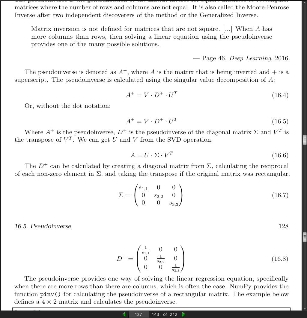
page 128:

• The pseudoinverse provides one way of solving the linear regression equation, specifically when there are more rows than there are columns, which is often the case. NumPy provides the function pinv() for calculating the pseudoinverse of a rectangular matrix.

>>> # pseudoinverse
>>> from numpy import array
>>> from numpy.linalg import pinv
>>> # define matrix
>>> A = array([
>>> [0.1, 0.2],
>>> [0.3, 0.4],
>>> [0.5, 0.6],
>>> [0.7, 0.8]])
>>> print(A)
[[0.1 0.2]
 [0.3 0.4]
 [0.5 0.6]
 [0.7 0.8]]

>>> # calculate pseudoinverse
>>> B = pinv(A)
>>> print(B)
[[ -1.00000000e+01 -5.00000000e+00 9.04289323e-15  5.00000000e+00]
 [  8.50000000e+00  4.50000000e+00 5.00000000e-01 -3.50000000e+00]]

page 129:

• We can calculate the pseudoinverse manually via the SVD and compare the results to the pinv() function. First we must calculate the SVD. Next we must calculate the reciprocal of each value in the s array. Then the s array can be transformed into a diagonal matrix with an added row of zeros to make it rectangular. Finally, we can calculate the pseudoinverse from the elements. The specific implementation is:

A^+ = V^T D^T U^T

>>># pseudoinverse via svd
>>>from numpy import array
>>>from numpy.linalg import svd
>>>from numpy import zeros
>>>from numpy import diag
>>># define matrix
>>>A = array([
>>>[0.1, 0.2],
>>>[0.3, 0.4],
>>>[0.5, 0.6],
>>>[0.7, 0.8]])
>>>print(A)
[[0.1 0.2]
 [0.3 0.4]
 [0.5 0.6]
 [0.7 0.8]]

>>> # factorize
>>> U, s, V = svd(A)
>>> # reciprocals of s
>>> d = 1.0 / s
>>> # create m x n D matrix
>>> D = zeros(A.shape)
>>> # populate D with n x n diagonal matrix
>>> D[:A.shape[1], :A.shape[1]] = diag(d)
>>> # calculate pseudoinverse
>>> B = V.T.dot(D.T).dot(U.T)
>>> print(B)
[[ -1.00000000e+01 -5.00000000e+00 9.04831765e-15  5.00000000e+00]
[   8.50000000e+00  4.50000000e+00 5.00000000e-01 -3.50000000e+00]]

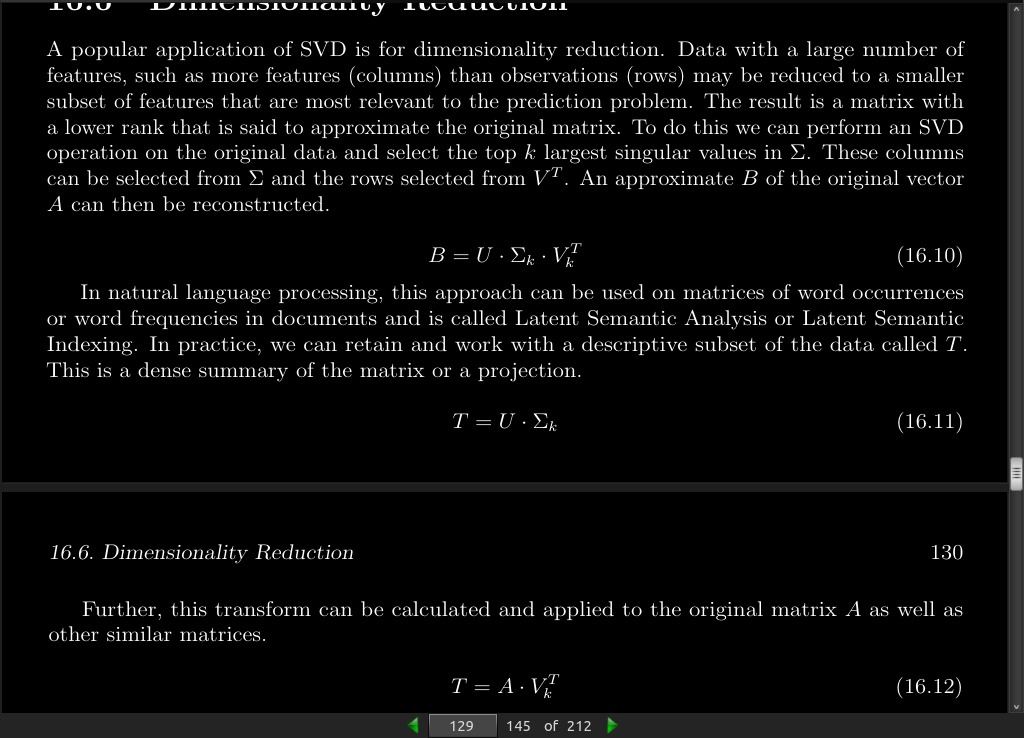
• A popular application of SVD is for dimensionality reduction. Data with a large number of features, such as more features (columns) than observations (rows) may be reduced to a smaller subset of features that are most relevant to the prediction problem. The result is a matrix with a lower rank that is said to approximate the original matrix. To do this we can perform an SVD operation on the original data and select the top k largest singular values in Σ. These columns can be selected from Σ and the rows selected from V T . An approximate B of the original vector A can then be reconstructed.

B = U · Σ_k · V_k^T  (16.10)

page 130:

• The example below demonstrates data reduction with the SVD. First a 3 × 10 matrix is defined, with more columns than rows. The SVD is calculated and only the first two features are selected. The elements are recombined to give an accurate reproduction of the original matrix. Finally the transform is calculated two different ways.

>>> # data reduction with svd
>>> from numpy import array
>>> from numpy import diag
>>> from numpy import zeros
>>> from scipy.linalg import svd
>>> # define matrix
>>> A = array([
>>> [1,2,3,4,5,6,7,8,9,10],
>>> [11,12,13,14,15,16,17,18,19,20],
>>> [21,22,23,24,25,26,27,28,29,30]])
>>> print(A)
[[ 1  2  3  4  5  6  7  8  9 10]
 [11 12 13 14 15 16 17 18 19 20]
 [21 22 23 24 25 26 27 28 29 30]]

>>> # factorize
>>> U, s, V = svd(A)
>>> # create m x n Sigma matrix
>>> Sigma = zeros((A.shape[0], A.shape[1]))
>>> # populate Sigma with n x n diagonal matrix
>>> Sigma[:A.shape[0], :A.shape[0]] = diag(s)
>>> # select
>>> n_elements = 2
>>> Sigma = Sigma[:, :n_elements]
>>> V = V[:n_elements, :]
>>> # reconstruct
>>> B = U.dot(Sigma.dot(V))
>>> print(B)
[[ 1.   2.  3.  4.  5.  6.  7.  8.  9. 10.]
 [ 11. 12. 13. 14. 15. 16. 17. 18. 19. 20.]
 [ 21. 22. 23. 24. 25. 26. 27. 28. 29. 30.]]

>>> # transform
>>> T = U.dot(Sigma)
>>> print(T)
[[-18.52157747  6.47697214]
 [-49.81310011  1.91182038]
 [-81.10462276 -2.65333138]]

>>> T = A.dot(V.T)
>>> print(T)
[[-18.52157747  6.47697214]
 [-49.81310011  1.91182038]
 [-81.10462276 -2.65333138]]

page 131:

• The scikit-learn provides a TruncatedSVD class that implements this capability directly. The TruncatedSVD class can be created in which you must specify the number of desirable features or components to select, e.g. 2. Once created, you can fit the transform (e.g. calculate Vk T ) by calling the fit() function, then apply it to the original matrix by calling the transform() function. The result is the transform of A called T above. The example below demonstrates the TruncatedSVD class.

>>> # svd data reduction in scikit-learn
>>> from numpy import array
>>> from sklearn.decomposition import TruncatedSVD
>>> # define matrix
>>> A = array([
>>> [1,2,3,4,5,6,7,8,9,10],
>>> [11,12,13,14,15,16,17,18,19,20],
>>> [21,22,23,24,25,26,27,28,29,30]])
>>> print(A)
[[ 1  2  3  4  5  6  7  8  9 10]
 [11 12 13 14 15 16 17 18 19 20]
 [21 22 23 24 25 26 27 28 29 30]]

>>> # create transform
>>> svd = TruncatedSVD(n_components=2)
>>> # fit transform
>>> svd.fit(A)
>>> # apply transform
>>> result = svd.transform(A)
>>> print(result)
[[ 18.52157747  6.47697214]
 [ 49.81310011  1.91182038]
 [ 81.10462276 -2.65333138]]

• We can see that the values match those calculated manually above, except for the sign on some values. We can expect there to be some instability when it comes to the sign given the nature of the calculations involved and the differences in the underlying libraries and methods used. This instability of sign should not be a problem in practice as long as the transform is trained for reuse.

Part 6: Statistics

· 17: Introduction to Multivariate Statistics

page 138:

>>> # matrix means
>>> from numpy import array
>>> from numpy import mean
>>> # define matrix
>>> M = array([
>>> [1,2,3,4,5,6],
>>> [1,2,3,4,5,6]])
>>> print(M)
[[1 2 3 4 5 6]
 [1 2 3 4 5 6]]

>>> # column means
>>> col_mean = mean(M, axis=0)
>>> print(col_mean)
[1. 2. 3. 4. 5. 6.]

>>> # row means
>>> row_mean = mean(M, axis=1)
>>> print(row_mean)
[3.5 3.5]

page 139:

• sample variance is denoted by the lower case sigma with a 2 superscript indicating the units are squared (e.g. σ^2 ), not that you must square the final value.

• In NumPy, the variance can be calculated for a vector or a matrix using the var() function. By default, the var() function calculates the population variance. To calculate the sample variance, you must set the ddof argument to the value 1. The example below defines a 6-element vector and calculates the sample variance.

>>> # vector variance
>>> from numpy import array
>>> from numpy import var
>>> # define vector
>>> v = array([1,2,3,4,5,6])
>>> print(v)
[1 2 3 4 5 6]

>>> # calculate variance
>>> result = var(v, ddof=1)
>>> print(result)
3.5

page 140:

>>> # matrix variances
>>> from numpy import array
>>> from numpy import var
>>> # define matrix
>>> M = array([
>>> [1,2,3,4,5,6],
>>> [1,2,3,4,5,6]])
>>> print(M)
[[1 2 3 4 5 6]
 [1 2 3 4 5 6]]

>>> # column variances
>>> col_var = var(M, ddof=1, axis=0)
>>> print(col_var)
[ 0. 0. 0. 0. 0. 0.]

>>> # row variances
>>> row_var = var(M, ddof=1, axis=1)
>>> print(row_var)
[ 3.5 3.5]

• The standard deviation is calculated as the square root of the variance and is denoted as lowercase s.

s = √σ2

• NumPy also provides a function for calculating the standard deviation directly via the std() function. As with the var() function, the ddof argument must be set to 1 to calculate the unbiased sample standard deviation and column and row standard deviations can be calculated by setting the axis argument to 0 and 1 respectively. The example below demonstrates how to calculate the sample standard deviation for the rows and columns of a matrix.

>>> # matrix standard deviation
>>> from numpy import array
>>> from numpy import std
>>> # define matrix
>>> M = array([
>>> [1,2,3,4,5,6],
>>> [1,2,3,4,5,6]])
>>> print(M)
[[1 2 3 4 5 6]
 [1 2 3 4 5 6]]

>>> # column standard deviations
>>> col_std = std(M, ddof=1, axis=0)
>>> print(col_std)
[0. 0. 0. 0. 0. 0.]

>>> # row standard deviations
>>> row_std = std(M, ddof=1, axis=1)
>>> print(row_std)
[1.87082869 1.87082869]

• In probability, covariance is the measure of the joint probability for two random variables. It describes how the two variables change together. It is denoted as the function cov(X,Y), where X and Y are the two random variables being considered.

page 141:

• NumPy does not have a function to calculate the covariance between two variables directly. Instead, it has a function for calculating a covariance matrix called cov() that we can use to retrieve the covariance. By default, the cov() function will calculate the unbiased or sample covariance between the provided random variables.

page 142:

• The covariance can be normalized to a score between -1 and 1 to make the magnitude interpretable by dividing it by the standard deviation of X and Y . The result is called the correlation of the variables, also called the Pearson correlation coefficient, named for the developer of the method.

r = cov(X,Y) / (sX × sY)  (17.17)

• NumPy provides the corrcoef() function for calculating the correlation between two variables directly.

>>> # vector correlation
>>> from numpy import array
>>> from numpy import corrcoef
>>> # define first vector
>>> x = array([1,2,3,4,5,6,7,8,9])
>>> print(x)
[1 2 3 4 5 6 7 8 9]

>>> # define second vector
>>> y = array([9,8,7,6,5,4,3,2,1])
>>> print(y)
[9 8 7 6 5 4 3 2 1]

>>> # calculate correlation
>>> corr = corrcoef(x,y)[0,1]
>>> print(corr)
-1.0

page 143:

• The covariance matrix is a square and symmetric matrix that describes the covariance between two or more random variables. The diagonal of the covariance matrix are the variances of each of the random variables, as such it is often called the variance-covariance matrix.

• It is a key element used in the Principal Component Analysis data reduction method, or PCA for short. The covariance matrix can be calculated in NumPy using the cov() function. By default, this function will calculate the sample covariance matrix. The cov() function can be called with a single 2D array where each sub-array contains a feature (e.g. column). If this function is called with your data defined in a normal matrix format (rows then columns), then a transpose of the matrix will need to be provided to the function in order to correctly calculate the covariance of the columns.

>>># covariance matrix
>>>from numpy import array
>>>from numpy import cov
>>># define matrix of observations
>>>X = array([
>>>[1, 5, 8],
>>>[3, 5, 11],
>>>[2, 4, 9],
>>>[3, 6, 10],
>>>[1, 5, 10]])
>>>print(X)
[[1, 5, 8],
 [3, 5, 11],
 [2, 4, 9],
 [3, 6, 10],
 [1, 5, 10]]

>>> # calculate covariance matrix
>>> Sigma = cov(X.T)
>>> print(Sigma)
[[ 1.   0.25 0.75]
 [ 0.25 0.5  0.25]
 [ 0.75 0.25 1.3 ]]

· 18: Principal Component Analysis

page 148:

page 149:

# principal component analysis
from numpy import array
from numpy import mean
from numpy import cov
from numpy.linalg import eig
# define matrix
A = array([
[1, 2],
[3, 4],
[5, 6]])
print(A)
[[1, 2],
 [3, 4],
 [5, 6]]

# column means
M = mean(A.T, axis=1)
# center columns by subtracting column means
C = A - M
# calculate covariance matrix of centered matrix
V = cov(C.T)
# factorize covariance matrix
values, vectors = eig(V)
print(vectors)
[[ 0.70710678 -0.70710678]
 [ 0.70710678  0.70710678]]

print(values)
[8. 0.]

# project data
P = vectors.T.dot(C.T)
print(P.T)
[[-2.82842712 0. ]
 [ 0.         0. ]
 [ 2.82842712 0. ]]

• Running the example first prints the original matrix, then the eigenvectors and eigenvalues of the centered covariance matrix, followed finally by the projection of the original matrix. Interestingly, we can see that only the first eigenvector is required, suggesting that we could project our 3 × 2 matrix onto a 3 × 1 matrix with little loss.

page 150:

• We can calculate a Principal Component Analysis on a dataset using the PCA() class in the scikit-learn library. The benefit of this approach is that once the projection is calculated, it can be applied to new data again and again quite easily. When creating the class, the number of components can be specified as a parameter. The class is first fit on a dataset by calling the fit() function, and then the original dataset or other data can be projected into a subspace with the chosen number of dimensions by calling the transform() function. Once fit, the singular values and principal components can be accessed on the PCA class via the explained_variance_ and components_attributes_.

>>> # principal component analysis with scikit-learn
>>> from numpy import array
>>> from sklearn.decomposition import PCA
>>> # define matrix
>>> A = array([
>>> [1, 2],
>>> [3, 4],
>>> [5, 6]])
>>> print(A)
[[1, 2],
 [3, 4],
 [5, 6]]

>>> # create the transform
>>> pca = PCA(2)
>>> # fit transform
>>> pca.fit(A)
>>> # access values and vectors
>>> print(pca.components_)
[[ 0.70710678  0.70710678]
 [ 0.70710678 -0.70710678]]

>>> print(pca.explained_variance_)
[ 8.00000000e+00 2.25080839e-33]

>>> # transform data
>>> B = pca.transform(A)
>>> print(B)
[[ -2.82842712e+00  2.22044605e-16]
 [  0.00000000e+00  0.00000000e+00]
 [  2.82842712e+00 -2.22044605e-16]]

· 19: Linear Regression

page 155:

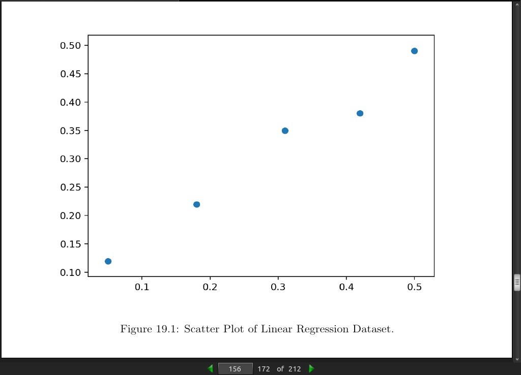
>>> # linear regression dataset
>>> from numpy import array
>>> from matplotlib import pyplot
>>> # define dataset
>>> data = array([
>>> [0.05, 0.12],
>>> [0.18, 0.22],
>>> [0.31, 0.35],
>>> [0.42, 0.38],
>>> [0.5, 0.49]])
>>> print(data)
[[0.05, 0.12],
 [0.18, 0.22],
 [0.31, 0.35],
 [0.42, 0.38],
 [0.5, 0.49]]

>>> # split into inputs and outputs
>>> X, y = data[:,0], data[:,1]
>>> X = X.reshape((len(X), 1))
>>> # scatter plot
>>> pyplot.scatter(X, y)
>>> pyplot.show()
[[0.05 0.12]
 [0.18 0.22]
 [0.31 0.35]
 [0.42 0.38]
 [0.5  0.49]]

page 156:

page 157:

>>> # direct solution to linear least squares
>>> from numpy import array
>>> from numpy.linalg import inv
>>> from matplotlib import pyplot
>>> # define dataset
>>> data = array([
>>> [0.05, 0.12],
>>> [0.18, 0.22],
>>> [0.31, 0.35],
>>> [0.42, 0.38],
>>> [0.5, 0.49]])

>>> # split into inputs and outputs
>>> X, y = data[:,0], data[:,1]
>>> X = X.reshape((len(X), 1))
>>> # linear least squares
>>> b = inv(X.T.dot(X)).dot(X.T).dot(y)
>>> print(b)
[1.00233226]

>>> # predict using coefficients
>>> yhat = X.dot(b)

>>> # plot data and predictions
>>> pyplot.scatter(X, y)
>>> pyplot.plot(X, yhat, color=✬red✬)
>>> pyplot.show()

page 158:

• A problem with this approach is the matrix inverse that is both computationally expensive and numerically unstable. An alternative approach is to use a matrix decomposition to avoid this operation. We will look at two examples in the following sections.

• The QR decomposition is an approach of breaking a matrix down into its constituent elements.

A = Q · R  (19.13)

• Where A is the matrix that we wish to decompose, Q a matrix with the size m × m, and R is an upper triangle matrix with the size m × n. The QR decomposition is a popular approach for solving the linear least squares equation. Stepping over all of the derivation, the coefficients can be found using the Q and R elements as follows:

b = R^−1 · Q^T · y  (19.14)

• The approach still involves a matrix inversion, but in this case only on the simpler R matrix. The QR decomposition can be found using the qr() functionin NumPy. The calculation of the coefficients in NumPy looks as follows:

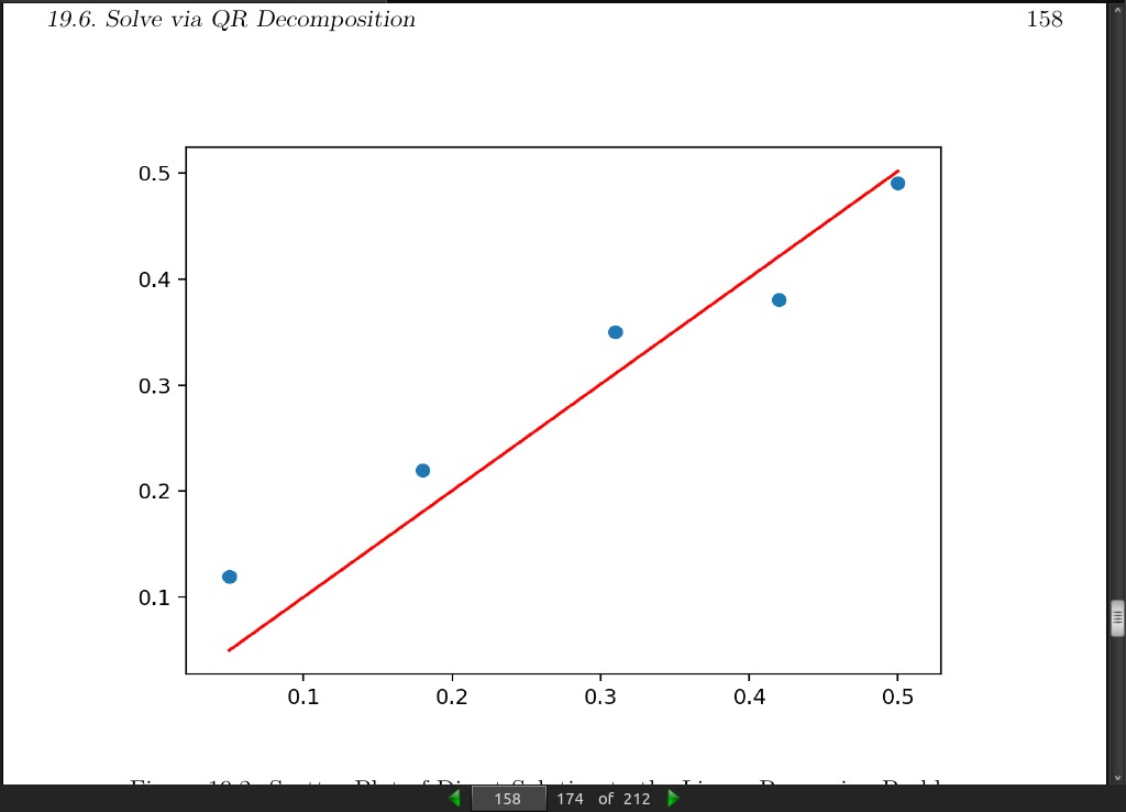
>>> # QR decomposition solution to linear least squares
>>> from numpy import array
>>> from numpy.linalg import inv
>>> from numpy.linalg import qr
>>> from matplotlib import pyplot
>>> # define dataset
>>> data = array([
>>> [0.05, 0.12],
>>> [0.18, 0.22],
>>> [0.31, 0.35],
>>> [0.42, 0.38],
>>> [0.5, 0.49]])
>>> # split into inputs and outputs

>>> X, y = data[:,0], data[:,1]
>>> X = X.reshape((len(X), 1))

>>> # factorize
>>> Q, R = qr(X)
>>> b = inv(R).dot(Q.T).dot(y)
>>> print(b)
[1.00233226]

>>> # predict using coefficients
>>> yhat = X.dot(b)

>>> # plot data and predictions
>>> pyplot.scatter(X, y)
>>> pyplot.plot(X, yhat, color=✬red✬)
>>> pyplot.show()

page 159:

• The QR decomposition approach is more computationally efficient and more numerically stable than calculating the normal equation directly, but does not work for all data matrices.

page 160:

• The Singular-Value Decomposition, or SVD for short, is a matrix decomposition method like the QR decomposition.

X = U Σ V^T  (19.15)

• Where A is the real n × m matrix that we wish to decompose, U is a m × m matrix, Σ (often represented by the uppercase Greek letter Sigma) is an m × n diagonal matrix, and V^T is the transpose of an n × n matrix. Unlike the QR decomposition, all matrices have a singular-value decomposition. As a basis for solving the system of linear equations for linear regression, SVD is more stable and the preferred approach. Once decomposed, the coefficients can be found by calculating the pseudoinverse of the input matrix X and multiplying that by the output vector y.

b = X^+ y  (19.16)

Where the pseudoinverse X + is calculated as following:

X^+ = U D^+ V^T  (19.17)

• Where X^+ is the pseudoinverse of X and the + is a superscript, D+ is the pseudoinverse of the diagonal matrix Σ and V^T is the transpose of V. NumPy provides the function pinv() to calculate the pseudoinverse directly.

>>> # SVD solution via pseudoinverse to linear least squares
>>> from numpy import array
>>> from numpy.linalg import pinv
>>> from matplotlib import pyplot
>>> # define dataset
>>> data = array([
>>> [0.05, 0.12],
>>> [0.18, 0.22],
>>> [0.31, 0.35],
>>> [0.42, 0.38],
>>> [0.5, 0.49]])

>>> # split into inputs and outputs
>>> X, y = data[:,0], data[:,1]
>>> X = X.reshape((len(X), 1))
>>> # calculate coefficients
>>> b = pinv(X).dot(y)
>>> print(b)
[ 1.00233226]

>>> # predict using coefficients
>>> yhat = X.dot(b)
>>> # plot data and predictions
>>> pyplot.scatter(X, y)
>>> pyplot.plot(X, yhat, color=✬red✬)
>>> pyplot.show()

page 162:

• The pseudoinverse via SVD approach to solving linear least squares is the de facto standard. This is because it is stable and works with most datasets. NumPy provides a convenience function named lstsq() that solves the linear least squares function using the SVD approach. The function takes as input the X matrix and y vector and returns the b coefficients as well as residual errors, the rank of the provided X matrix and the singular values.

>>> # least squares via convenience function
>>> from numpy import array
>>> from numpy.linalg import lstsq
>>> from matplotlib import pyplot
>>> # define dataset
>>> data = array([
>>> [0.05, 0.12],
>>> [0.18, 0.22],
>>> [0.31, 0.35],
>>> [0.42, 0.38],
>>> [0.5, 0.49]])

>>> # split into inputs and outputs
>>> X, y = data[:,0], data[:,1]
>>> X = X.reshape((len(X), 1))
>>> # calculate coefficients
>>> b, residuals, rank, s = lstsq(X, y)
>>> print(b)
[1.00233226]

>>> # predict using coefficients
>>> yhat = X.dot(b)
>>> # plot data and predictions
>>> pyplot.scatter(X, y)
>>> pyplot.plot(X, yhat, color=✬red✬)
>>> pyplot.show()

· Appendix

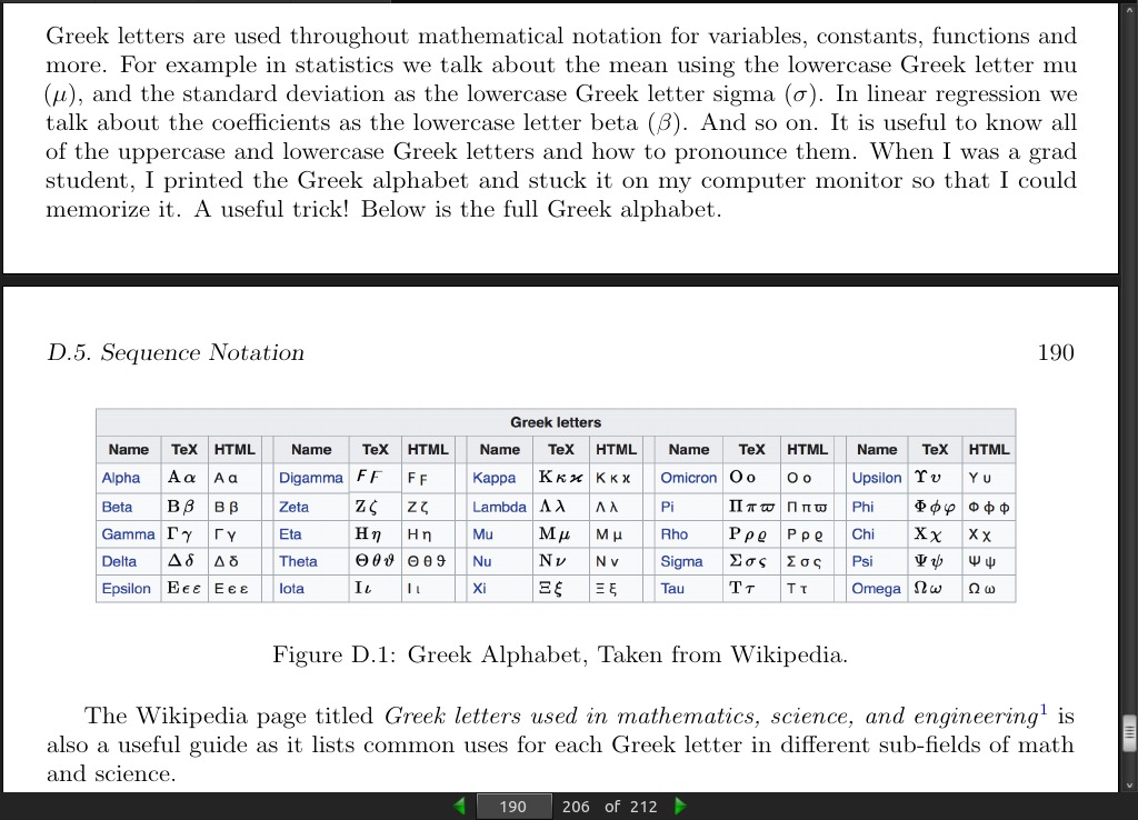
page 190: