Home · Projects · 2017 · Power Function Model
Published: July 9, 2017
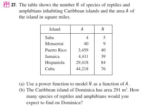
This is from a question in “Calculus Seventh Edition” by James Stewart. I have been using it to provide examples that I can work in python.
I’ve already lost the website that helped me sort this out by converting the data to log and then back again, but the scipy cookbook has a similar example (at the bottom of the page).
#!/usr/bin/env python
#Author: Mark Feineigle
#Create Date: 2017/06/30
# Model a power function
# Example: power_function_model.jpg
# From: CALCULUS SEVENTH EDITION JAMES STEWART
# Build xs and ys
# Convert xs and ys to log10
# Do linear regression on the log10 data
# Create sample data in log10
# m is the exponent and 10**b is the coefficient
# to solve you must convert the target value to log10
# and then to raise 10**result to get out of log10
import matplotlib.pyplot as plt
import numpy as np
from scipy import stats
# Build xs and ys
xs = np.array([4,
40,
3459,
4411,
29418,
44218,])
ys = np.array([5,
9,
40,
39,
84,
76,])
# Convert xs and ys to log10
logxs = np.log10(xs)
logys = np.log10(ys)
# Linear regression
m, b, r_value, p_value, std_err = stats.linregress(logxs, logys)
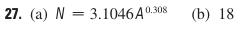
print m, 10**b # m is the exponent and 10**b is the coefficient
# m = 0.308044235477 10**b = 3.10462040171
answer = 10**(m*np.log10(291)+b) # prediction for 291
print answer
# answer = 17.8236456399
# Test data, in log10
samps = np.log10(np.arange(1,50000,1))
# plot in log and linear scales
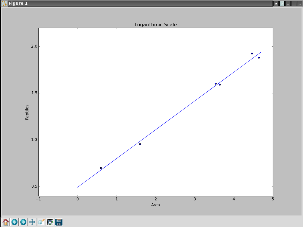
fig1 = plt.figure()
ax1 = fig1.add_subplot(111)
ax1.scatter(logxs, logys) # in log scale
ax1.loglog(samps, m*samps+b)
plt.title("Logarithmic Scale")
plt.xlabel("Island Area")
plt.ylabel("Reptiles")
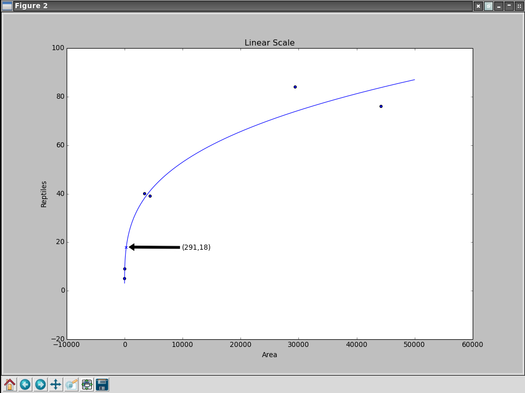
fig2 = plt.figure()
ax2 = fig2.add_subplot(111)
ax2.scatter(xs, ys)
ax2.plot(10**samps, 10**(m*samps+b)) # convert to linear
ax2.scatter(291, answer, marker="x")
plt.title("Linear Scale")
plt.xlabel("Island Area")
plt.ylabel("Reptiles")
plt.annotate("(291,18)", xy=(291,18), xytext=(10000,17),
arrowprops=dict(facecolor='black', shrink=0.05))
plt.show()