Home · Book Reports · 2018 · Python - Deeper Insights Into Machine Learning

Published: April 8, 2018 (5 years ago.)

Tags: Machine Learning · Programming · Python

Author :: Sebastian Raschka, David Julian, John Hearty

Publication Year :: 2016

Read Date :: 2018-04-08

Source :: Python__Deeper_Insights_into_Machine_Learning.pdf

The book in...

One sentence:

A great introduction that ramps up, through three modules with plenty of detailed code examples, to more advanced coverage of many aspects of machine learning.

Five sentences:

This is a straightforward, no nonsense book, or three, that will allow you to go from zero understanding of machine learning to quite advanced, assuming you put in the required time and effort. The code provided is detailed, extremely well explained, often line-by-line, and gives you a solid intuitive basis that will make your journey into the more advanced areas more concrete. The book starts slowly and then moves forward at a steady, but more than manageable, pace, building on the previous, often simplified examples using SKLearn, to reach more modern and advanced techniques using libraries such as Theano and Keras to leverage your GPU. It lacks some of the detail you might want when it comes to mathematical proofs, but it does include plenty math to whet your appetite; supplementing this book with a follow up with an appropriate linear algebra/algorithms math book would probably be ideal. Lastly, at the end of each chapter in the third module there are numerous resources provided for further study in regard to the more advanced topics.

designates my notes. / designates important.

Thoughts

Overall a great book. Would recommend to anyone interested in learning about machine learning.

It is basically 3 books in 1, separated, unsurprisingly, into beginner, intermediate, and advanced modules.

The detailed table of contents wins points with me every time.

The first book holds your hand and offers a very nice, slow, place to start. Compared to the other pair of beginner books I’ve read on the subject, this one was far superior.

All of the code works, which I can’t say about the other books, and there is often a line-by-line explanation following each snippet.

While there isn’t much in the way of real mathematical proofs, there is still plenty of math and what the underlying algorithms look like and do. Any understanding will help over simply using sklearn blindly. This said, after you have some intuitive understanding of what to expect when using various algorithms and libraries, you will be better equipped to tackle a more detailed and abstract exploration of the underlying mathematical underpinnings.

The second book goes back over the same ideas as the first book, but in more detail and with added depth. Great reinforcement learning. Practice, practice, practice!

Book three is considerably more advanced. It assumes you have the stuff from books one and two down pat. It uses the Theano and Keras libraries, which I didn’t have installed so I didn’t play with the code. The little bit of the code I did experiment with had numerous errors. This module included more advanced topics than I was ready for, but it was interesting none-the-less to expand my grammar for now.

Finally, there are tons of references to follow up and expand your understanding of whatever topic may suit your fancy. Again, all in all a great place to start if combined with another more mathematically oriented book.

Other

Google’s DeepDream program, which became well-known for its overtrained, hallucinogenic imagery, also uses a convolutional neural network.
“I suppose it is tempting, if the only tool you have is a hammer, to treat everything as if it were a nail” (Abraham Maslow, 1966) really, Maslow said this? note, I can’t get away from these assholes!

I would like a more detailed explanation of what is going on here, but, since it is matplotlib that I am not understanding, the lack of explanation can be forgiven. It plots the colored regions of the plots; I’m not sure what the meshgrid function is doing.

# plot the decision surface
x1_min, x1_max = X[:, 0].min() - 1, X[:, 0].max() + 1
x2_min, x2_max = X[:, 1].min() - 1, X[:, 1].max() + 1
xx1, xx2 = np.meshgrid(np.arange(x1_min, x1_max, resolution),
                       np.arange(x2_min, x2_max, resolution))
Z = classifier.predict(np.array([xx1.ravel(), xx2.ravel()]).T)
Z = Z.reshape(xx1.shape)
plt.contourf(xx1, xx2, Z, alpha=0.4, cmap=cmap)
plt.xlim(xx1.min(), xx1.max())
plt.ylim(xx2.min(), xx2.max())

Code Examples

Exceptional Excerpts

“This [The expression of emotion in 20th century books (Acerbi et al, 2013)] study is interesting for several reasons. Firstly, it is an example of data-driven science, where previously considered soft sciences, such as sociology and anthropology, are given a solid empirical footing."

“For data to become information, it requires some meaningful structure."

“fill in the missing values through a process of imputation. For classification, we can simply use the statistics of the mean, median, and mode over the observed features to impute the missing values."

“Many machine learning algorithms require that features are standardized. This means that they will work best when the individual features look more or less like normally distributed data with near-zero mean and unit variance. The easiest way to do this is by subtracting the mean value from each feature and scaling it by dividing by the standard deviation. This can be achieved by the scale() function or the standardScaler() function in the sklearn.preprocessing() function. Although these functions will accept sparse data, they probably should not be used in such situations because centering sparse data would likely destroy its structure. It is recommended to use the MacAbsScaler() or maxabs_scale() function in these cases. The former scales and translates each feature individually by its maximum absolute value. The latter scales each feature individually to a range of [-1,1]. Another specific case is when we have outliers in the data. In these cases using the robust_scale() or RobustScaler() function is recommended."

“Bagging is primarily a variance reduction technique and boosting is primarily a bias reduction technique."

“GoogLeNet was designed to tackle computer vision challenges involving Internet-quality image data, that is, images that have been captured in real contexts where the pose, lighting, occlusion, and clutter of images vary significantly. GoogLeNet was applied to the 2014 ImageNet challenge with noteworthy success, achieving only 6.7% error rate on the test dataset. ImageNet images are small, high-granularity images taken from many, varied classes."

Pages numbers from book.

Module 1: Python Machine Learning

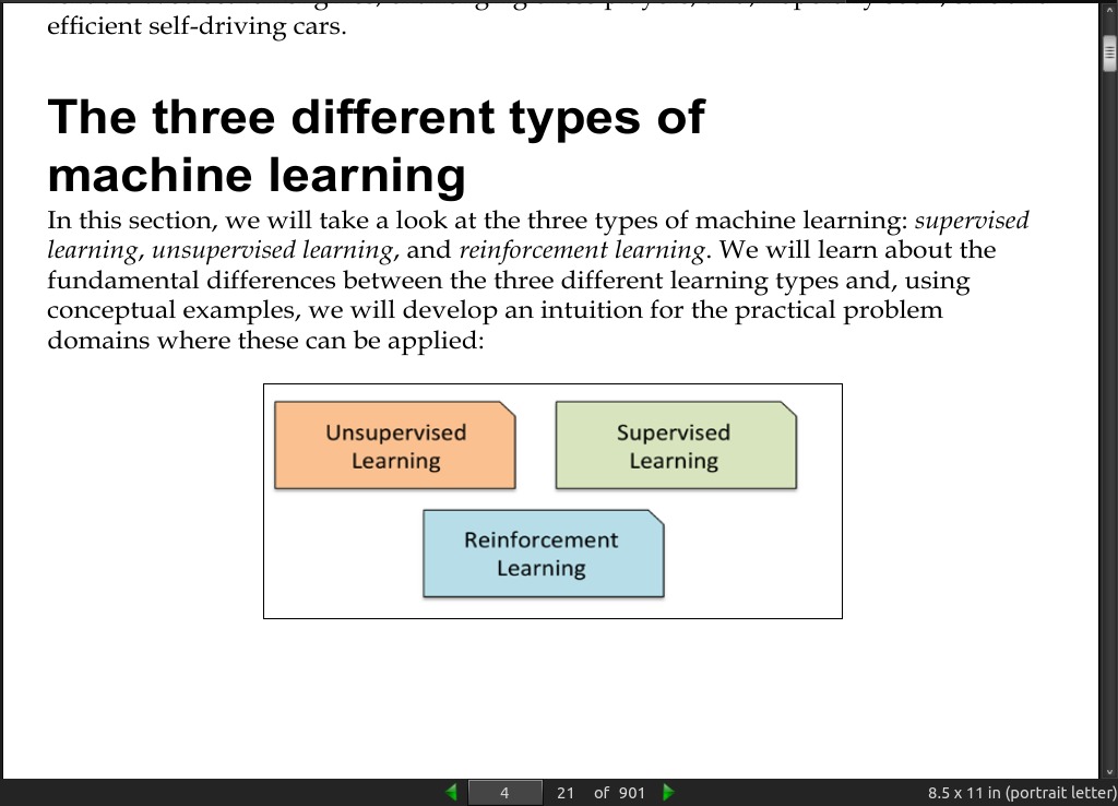
· 01: Giving Computers the Ability to Learn from Data

page 004:

page 010:

page 012:

page 14:

The Lack of A Priori Distinctions Between Learning Algorithms, (D.H. Wolpert

No Free Lunch Theorems for Optimization, (D.H. Wolpert and W.G. Macready,

“I suppose it is tempting, if the only tool you have is a hammer, to treat everything as if it were a nail” (Abraham Maslow, 1966)
hyperparameter optimization techniques that help us to fine-tune the performance of our model in later chapters. Intuitively, we can think of those hyperparameters as parameters that are not learned from the data but represent the knobs of a model that we can turn to improve its performance

· 02: Training Machine Learning Algorithms for Classification

page 24:

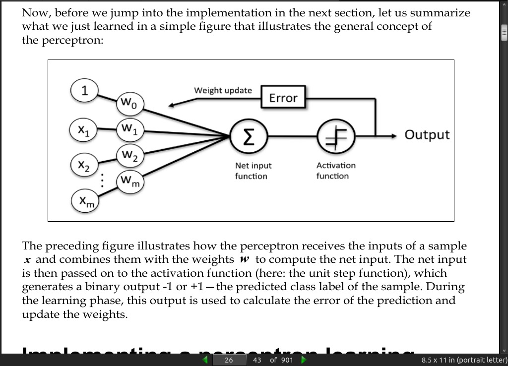
Easy to follow mathematics of perceptron.

page 25:

It is important to note that the convergence of the perceptron is only guaranteed if the two classes are linearly separable and the learning rate is sufficiently small.

page 026:

page 035:

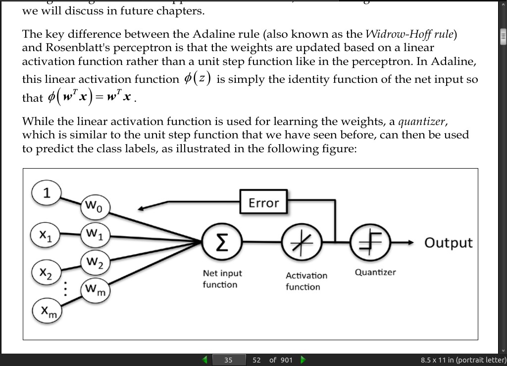
page 36:

(batch) gradient descent.

page 44:

stochastic gradient descent, sometimes also called iterative or on-line gradient descent

page 45:

To obtain accurate results via stochastic gradient descent, it is important to present it with data in a random order, which is why we want to shuffle the training set for every epoch to prevent cycles.
eta may be made to decrease over time in stochastic gradient descent.
Another advantage of stochastic gradient descent is that we can use it for online learning. In online learning, our model is trained on-the-fly as new training data arrives.
A compromise between batch gradient descent and stochastic gradient descent is the so-called mini-batch learning. Mini-batch learning can be understood as applying batch gradient descent to smaller subsets of the training data—for example, 50 samples at a time. The advantage over batch gradient descent is that convergence is reached faster via mini-batches because of the more frequent weight updates. Furthermore, mini-batch learning allows us to replace the for-loop over the training samples in Stochastic Gradient Descent (SGD) by vectorized operations, which can further improve the computational efficiency of our learning algorithm.

· 03: A Tour of Machine Learning Classifiers Using Scikit-learn

page 51:

In practice, it is always recommended that you compare the performance of at least a handful of different learning algorithms to select the best model for the particular problem

page 52:

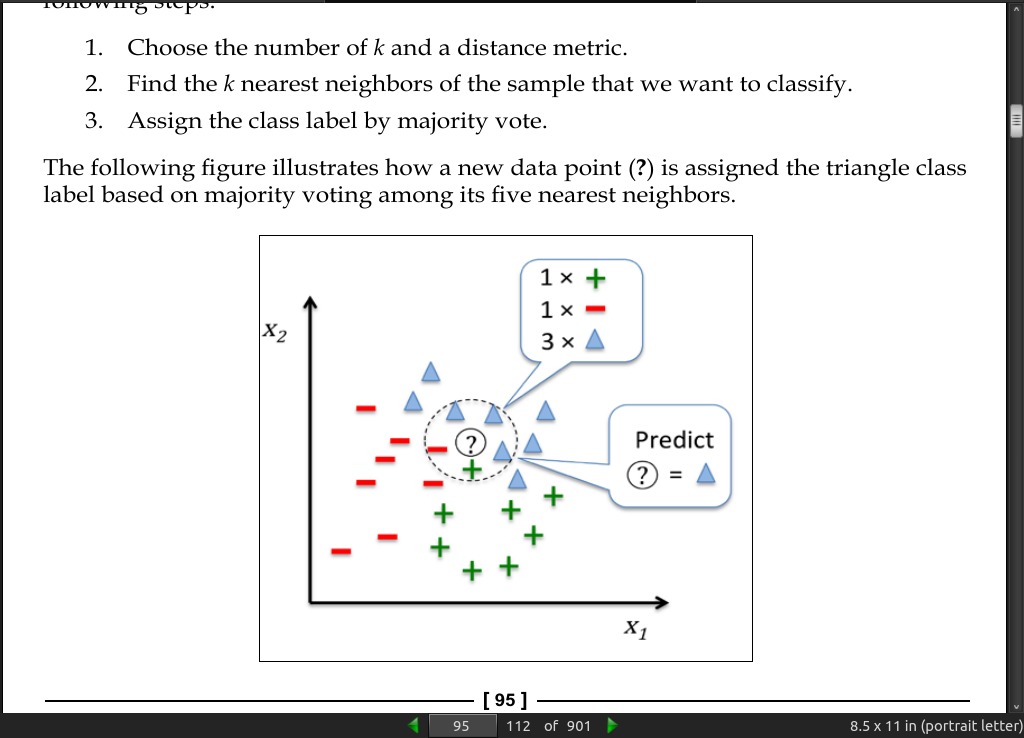
The five main steps that are involved in training a machine learning algorithm can be summarized as follows:

1.	 Selection of features.
2.	 Choosing a performance metric.
3.	 Choosing a classifier and optimization algorithm.
4.	 Evaluating the performance of the model.
5.	 Tuning the algorithm.

page 55:

Instead of the misclassification error, many machine learning practitioners report the classification accuracy of a model, which is simply calculated as follows:

if misclassification error = 0.089
1 - misclassification error = 0.911 or 91.1 percent.

page 60:

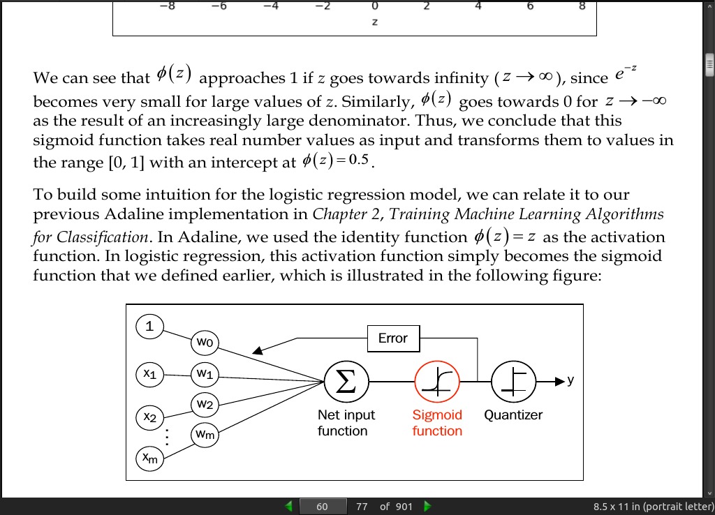
In logistic regression, this activation function simply becomes the sigmoid function that we defined earlier… The output of the sigmoid function is then interpreted as the probability of particular sample belonging to class 1

page 61:

Logistic regression is used in weather forecasting, for example, to not only predict if it will rain on a particular day but also to report the chance of rain. Similarly, logistic regression can be used to predict the chance that a patient has a particular disease given certain symptoms, which is why logistic regression enjoys wide popularity in the field of medicine.

page 68:

The concept behind regularization is to introduce additional information (bias) to penalize extreme parameter weights. The most common form of regularization is the so-called L2 regularization (sometimes also called L2 shrinkage or weight decay)
Regularization is another reason why feature scaling such as standardization is important. For regularization to work properly, we need to ensure that all our features are on comparable scales.

page 70:

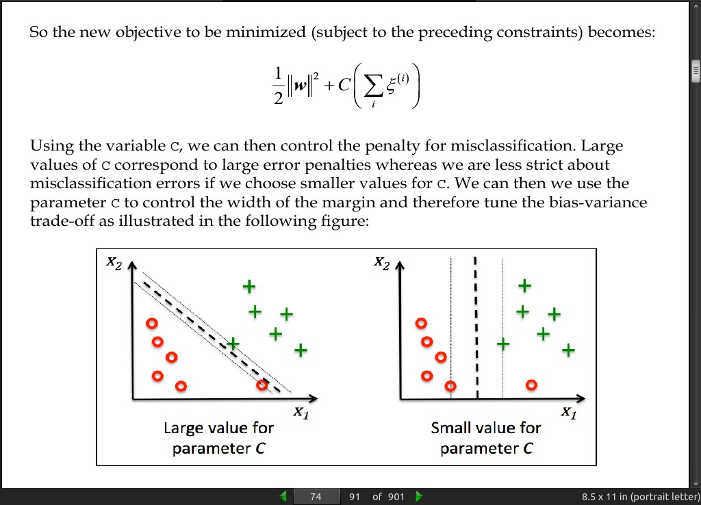
Consequently, decreasing the value of the inverse regularization parameter C means that we are increasing the regularization strength

page 71:

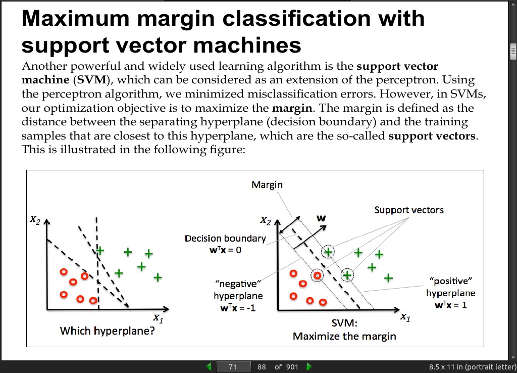
the support vector machine (SVM), which can be considered as an extension of the perceptron. Using the perceptron algorithm, we minimized misclassification errors. However, in SVMs, our optimization objective is to maximize the margin.

page 074:

page 76:

In practical classification tasks, linear logistic regression and linear SVMs often yield very similar results. Logistic regression tries to maximize the conditional likelihoods of the training data, which makes it more prone to outliers than SVMs. The SVMs mostly care about the points that are closest to the decision boundary (support vectors). On the other hand, logistic regression has the advantage that it is a simpler model that can be implemented more easily. Furthermore, logistic regression models can be easily updated, which is attractive when working with streaming data.
sometimes our datasets are too large to fit into computer memory. Thus, scikit-learn also offers alternative implementations via the SGDClassifier class, which also supports online learning via the partial_fit method. The concept behind the SGDClassifier class is similar to the stochastic gradient algorithm

>>> from sklearn.linear_model import SGDClassifier
>>> ppn = SGDClassifier(loss='perceptron')
>>> lr = SGDClassifier(loss='log')
>>> svm = SGDClassifier(loss='hinge')

page 078:

page 79:

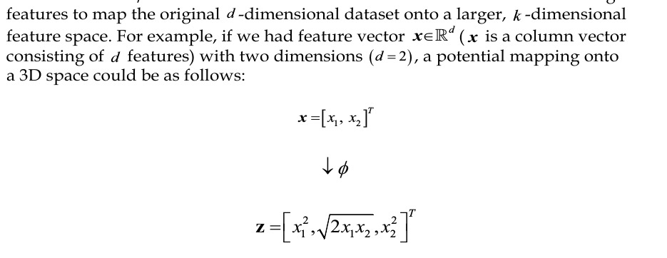
One of the most widely used kernels is the Radial Basis Function kernel (RBF kernel) or Gaussian kernel

page 84:

information gain is simply the difference between the impurity of the parent node and the sum of the child node impurities—the lower the impurity of the child nodes, the larger the information gain. However, for simplicity and to reduce the combinatorial search space, most libraries (including scikit-learn) implement binary decision trees. This means that each parent node is split into two child nodes
the three impurity measures or splitting criteria that are commonly used in binary decision trees are Gini impurity (I_G), entropy (I_H), and the classification error (I_E).

page 85:

However, in practice both the Gini impurity and entropy typically yield very similar results and it is often not worth spending much time on evaluating trees using different impurity criteria rather than experimenting with different pruning cut-offs.

page 86:

classification error is a useful criterion for pruning but not recommended for growing a decision tree, since it is less sensitive to changes in the class probabilities of the nodes.

page 94:

KNN (k-nearest neighbors) is a typical example of a lazy learner. It is called lazy not because of its apparent simplicity, but because it doesn’t learn a discriminative function from the training data but memorizes the training dataset instead.

page 95:

Parametric versus nonparametric models:
Machine learning algorithms can be grouped into parametric and nonparametric models. Using parametric models, we estimate parameters from the training dataset to learn a function that can classify new data points without requiring the original training dataset anymore. Typical examples of parametric models are the perceptron, logistic regression, and the linear SVM. In contrast, nonparametric models can’t be characterized by a fixed set of parameters, and the number of parameters grows with the training data. Two examples of nonparametric models that we have seen so far are the decision tree classifier/random forest and the kernel SVM.
KNN belongs to a subcategory of nonparametric models that is described as instance-based learning. Models based on instance-based learning are characterized by memorizing the training dataset, and lazy learning is a special case of instance-based learning that is associated with no (zero) cost during the learning process.

page 96:

The main advantage of such a memory-based approach is that the classifier immediately adapts as we collect new training data. However, the downside is that the computational complexity for classifying new samples grows linearly with the number of samples in the training dataset in the worst-case scenario
Furthermore, we can’t discard training samples since no training step is involved. Thus, storage space can become a challenge if we are working with large datasets.

page 98:

The curse of dimensionality = It is important to mention that KNN is very susceptible to overfitting due to the curse of dimensionality. The curse of dimensionality describes the phenomenon where the feature space becomes increasingly sparse for an increasing number of dimensions of a fixed-size training dataset. Intuitively, we can think of even the closest neighbors being too far away in a high-dimensional space to give a good estimate.
in models where regularization is not applicable such as decision trees and KNN, we can use feature selection and dimensionality reduction techniques to help us avoid the curse of dimensionality.

· 04: Building Good Training Sets – Data Preprocessing

page 103:

Although scikit-learn was developed for working with NumPy arrays, it can sometimes be more convenient to preprocess data using pandas’ DataFrame. We can always access the underlying NumPy array of the DataFrame via the values attribute before we feed it into a scikit-learn estimator:

>>> df.values
array([[ 1.,  2.,  3.,  4.],
       [ 5.,  6., nan,  8.],
       [10., 11., 12., nan]])

One of the easiest ways to deal with missing data is to simply remove the corresponding features (columns) or samples (rows) from the dataset entirely; rows with missing values can be easily dropped via the dropna method:

>>> df.dropna()
A B C D
0 1 2 3 4

Similarly, we can drop columns that have at least one NaN in any row by setting the axis argument to 1:

>>> df.dropna(axis=1)
A B
0 1 2
1 5 6
2 10 11

The dropna method supports several additional parameters that can come in handy:

# only drop rows where all columns are NaN
>>> df.dropna(how='all')
# drop rows that have not at least 4 non-NaN values
>>> df.dropna(thresh=4)
# only drop rows where NaN appear in specific columns (here: 'C')
>>> df.dropna(subset=['C'])

page 104:

One of the most common interpolation techniques is mean imputation, where we simply replace the missing value by the mean value of the entire feature column. A convenient way to achieve this is by using the Imputer class from scikit-learn,
The Imputer class belongs to the so-called transformer classes in scikit-learn that are used for data transformation. The two essential methods of those estimators are fit and transform. The fit method is used to learn the parameters from the training data, and the transform method uses those parameters to transform the data. Any data array that is to be transformed needs to have the same number of features as the data array that was used to fit the model.

page 105:

page 106:

Ordinal features can be understood as categorical values that can be sorted or ordered. For example, T-shirt size would be an ordinal feature, because we can define an order XL > L > M. In contrast, nominal features don’t imply any order and, to continue with the previous example, we could think of T-shirt color as a nominal feature since it typically doesn’t make sense to say that, for example, red is larger than blue.

page 112:

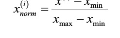
Now, there are two common approaches to bringing different features onto the same scale: normalization and standardization.
normalization refers to the rescaling of the features to a range of [0, 1], which is a special case of min-max scaling.

page 113:

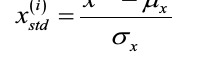
Using standardization, we center the feature columns at mean 0 with standard deviation 1 so that the feature columns take the form of a normal distribution, which makes it easier to learn the weights. Furthermore, standardization maintains useful information about outliers and makes the algorithm less sensitive to them in contrast to min-max scaling
Here, μ_x is the sample mean of a particular feature column and σ_x the corresponding standard deviation, respectively.

page 120:

There are two main categories of dimensionality reduction techniques: feature selection and feature extraction. Using feature selection, we select a subset of the original features. In feature extraction, we derive information from the feature set to construct a new feature subspace.

page 128:

However, as far as interpretability is concerned, the random forest technique comes with an important gotcha that is worth mentioning. For instance, if two or more features are highly correlated, one feature may be ranked very highly while the information of the other feature(s) may not be fully captured. On the other hand, we don’t need to be concerned about this problem if we are merely interested in the predictive performance of a model rather than the interpretation of feature importances.
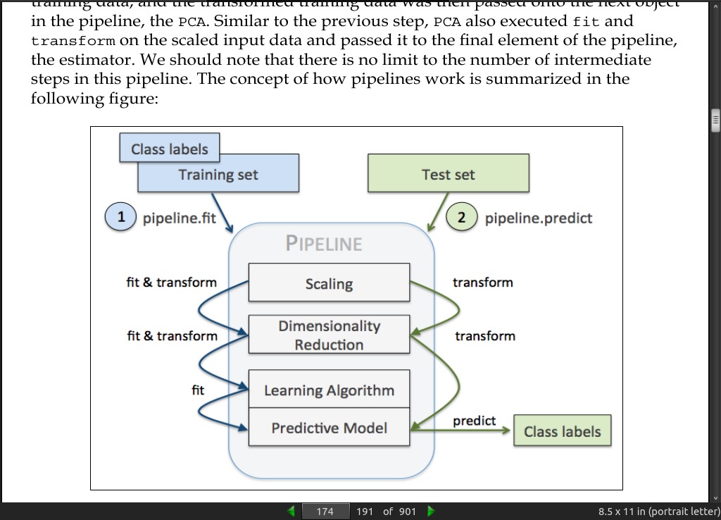
scikit-learn also implements a transform method that selects features based on a user-specified threshold after model fitting, which is useful if we want to use the RandomForestClassifier as a feature selector and intermediate step in a scikit-learn pipeline

· 05: Compressing Data via Dimensionality Reduction

page 130:

Feature extraction is typically used to improve computational efficiency but can also help to reduce the curse of dimensionality—especially if we are working with nonregularized models.
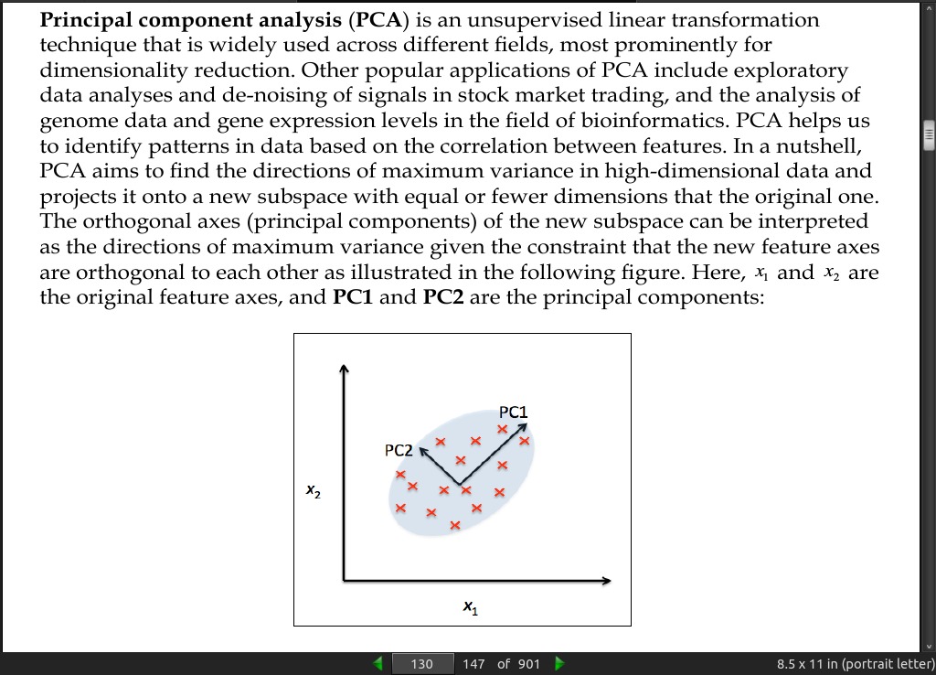
Principal component analysis (PCA) is an unsupervised linear transformation technique that is widely used across different fields, most prominently for dimensionality reduction.
PCA helps us to identify patterns in data based on the correlation between features. In a nutshell, PCA aims to find the directions of maximum variance in high-dimensional data and projects it onto a new subspace with equal or fewer dimensions that the original one.

page 131:

Note that the PCA directions are highly sensitive to data scaling, and we need to standardize the features prior to PCA if the features were measured on different scales and we want to assign equal importance to all features.

page 133:

Although the numpy.linalg.eig function was designed to decompose nonsymmetric square matrices, you may find that it returns complex eigenvalues in certain cases. A related function, numpy.linalg.eigh, has been implemented to decompose Hermetian matrices, which is a numerically more stable approach to work with symmetric matrices such as the covariance matrix; numpy.linalg.eigh always returns real eigenvalues.

page 140:

Linear Discriminant Analysis (LDA) can be used as a technique for feature extraction to increase the computational efficiency and reduce the degree of over-fitting due to the curse of dimensionality in nonregularized models.
Both LDA and PCA are linear transformation techniques that can be used to reduce the number of dimensions in a dataset; the former is an unsupervised algorithm, whereas the latter is supervised.

page 141:

One assumption in LDA is that the data is normally distributed. Also, we assume that the classes have identical covariance matrices and that the features are statistically independent of each other. However, even if one or more of those assumptions are slightly violated, LDA for dimensionality reduction can still work reasonably well

page 151:

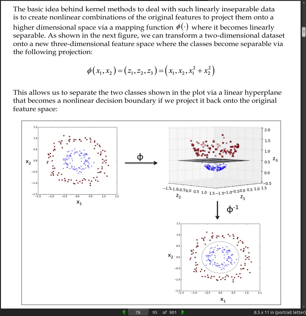
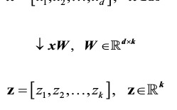
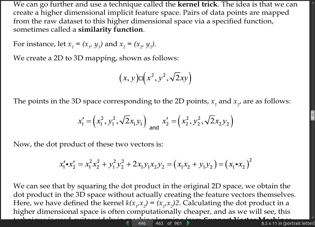
via kernel PCA we perform a nonlinear mapping that transforms the data onto a higher-dimensional space and use standard PCA in this higher-dimensional space to project the data back onto a lower-dimensional space

page 153:

Basically, the kernel function (or simply kernel) can be understood as a function that calculates a dot product between two vectors—a measure of similarity.

page 154:

page 169:

Using PCA, we projected data onto a lower-dimensional subspace to maximize the variance along the orthogonal feature axes while ignoring the class labels. LDA, in contrast to PCA, is a technique for supervised dimensionality reduction, which means that it considers class information in the training dataset to attempt to maximize the class-separability in a linear feature space. Lastly, you learned about a kernelized version of PCA, which allows you to map nonlinear datasets onto a lower-dimensional feature space where the classes become linearly separable.

· 06: Learning Best Practices for Model Evaluation and Hyperparameter Tuning

page 174:

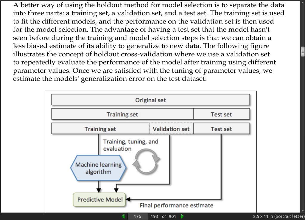
page 176:

A disadvantage of the holdout method is that the performance estimate is sensitive to how we partition the training set into the training and validation subsets; the estimate will vary for different samples of the data.

page 177:

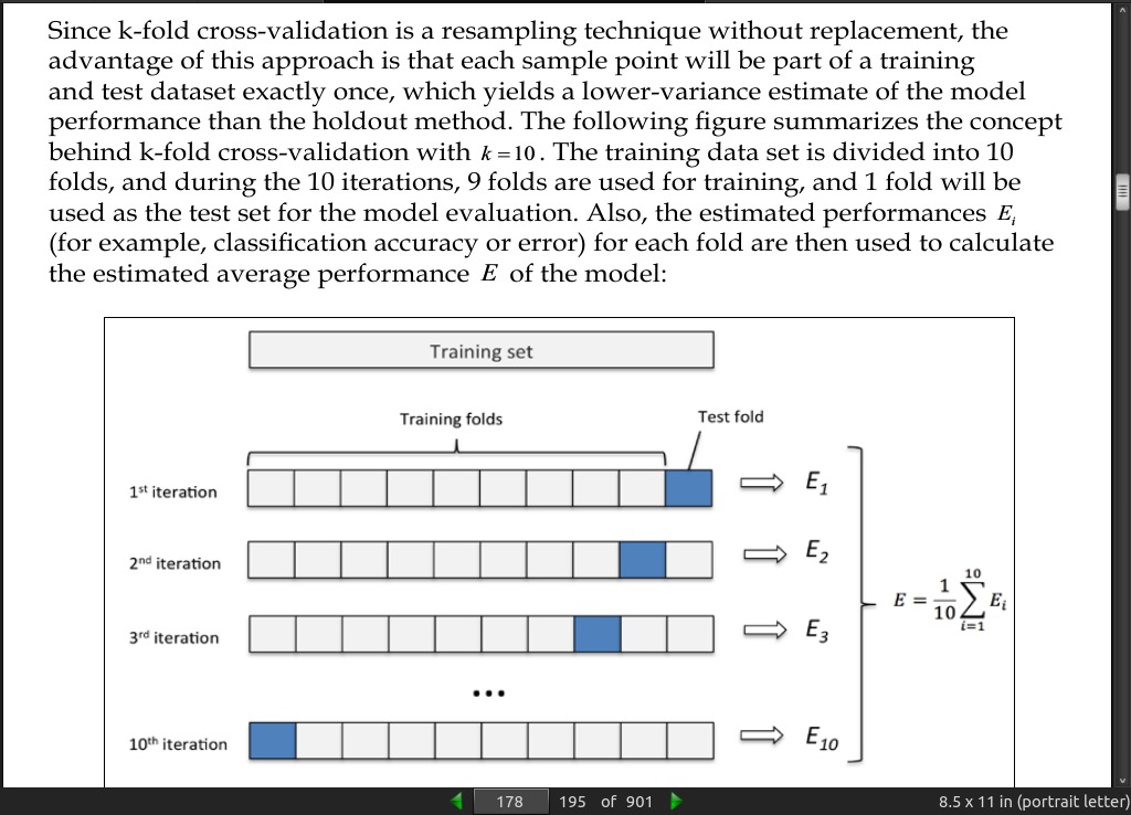
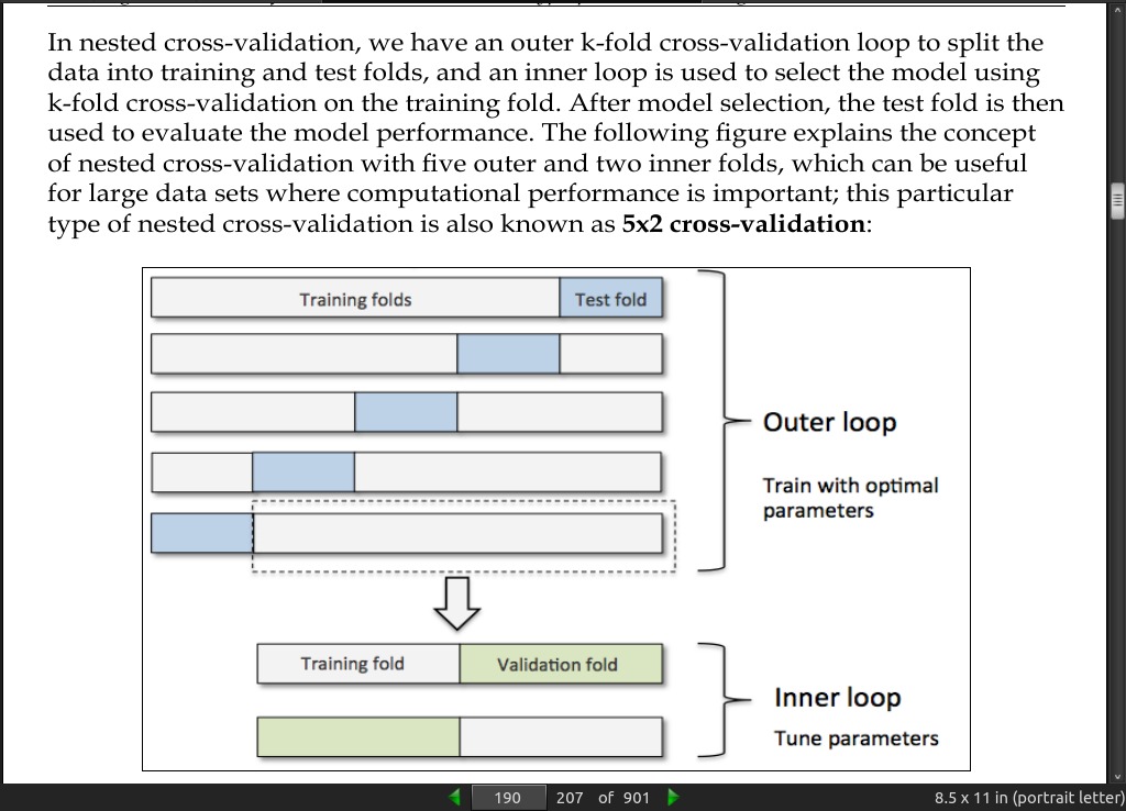
In k-fold cross-validation, we randomly split the training dataset into k folds without replacement, where k −1 folds are used for the model training and one fold is used for testing. This procedure is repeated k times so that we obtain k models and performance estimates.
In case you are not familiar with the terms sampling with and without replacement, let’s walk through a simple thought experiment. Let’s assume we are playing a lottery game where we randomly draw numbers from an urn. We start with an urn that holds five unique numbers 0, 1, 2, 3, and 4, and we draw exactly one number each turn. In the first round, the chance of drawing a particular number from the urn would be 1/5. Now, in sampling without replacement, we do not put the number back into the urn after each turn. Consequently, the probability of drawing a particular number from the set of remaining numbers in the next round depends on the previous round. For example, if we have a remaining set of numbers 0, 1, 2, and 4, the chance of drawing number 0 would become 1/4 in the next turn.
However, in random sampling with replacement, we always return the drawn number to the urn so that the probabilities of drawing a particular number at each turn does not change; we can draw the same number more than once. In other words, in sampling with replacement, the samples (numbers) are independent and have a covariance zero.

page 178:

The standard value for k in k-fold cross-validation is 10, which is typically a reasonable choice for most applications. However, if we are working with relatively small training sets, it can be useful to increase the number of folds. If we increase the value of k, more training data will be used in each iteration, which results in a lower bias towards estimating the generalization performance by averaging the individual model estimates. However, large values of k will also increase the runtime of the cross-validation algorithm and yield estimates with higher variance since the training folds will be more similar to each other. On the other hand, if we are working with large datasets, we can choose a smaller value for k, for example, k = 5 , and still obtain an accurate estimate of the average performance of the model while reducing the computational cost of refitting and evaluating the model on the different folds.

page 179:

In stratified cross-validation, the class proportions are preserved in each fold to ensure that each fold is representative of the class proportions in the training dataset,

page 182:

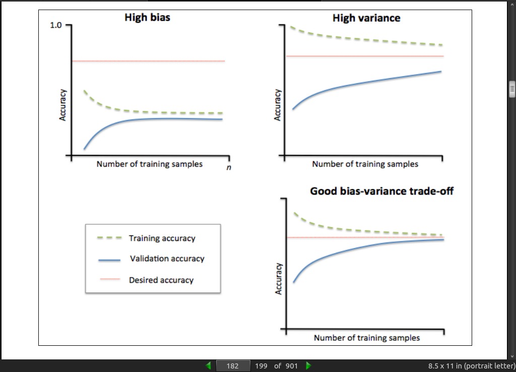
page 183:

The graph in the upper-left shows a model with high bias. This model has both low training and cross-validation accuracy, which indicates that it underfits the training data. Common ways to address this issue are to increase the number of parameters of the model, for example, by collecting or constructing additional features, or by decreasing the degree of regularization, for example, in SVM or logistic regression classifiers. The graph in the upper-right shows a model that suffers from high variance, which is indicated by the large gap between the training and cross-validation accuracy. To address this problem of overfitting, we can collect more training data or reduce the complexity of the model, for example, by increasing the regularization parameter; for unregularized models, it can also help to decrease the number of features via feature selection (Chapter 4, Building Good Training Sets – Data Preprocessing) or feature extraction (Chapter 5, Compressing Data via Dimensionality Reduction).

page 187:

In machine learning, we have two types of parameters: those that are learned from the training data, for example, the weights in logistic regression, and the parameters of a learning algorithm that are optimized separately. The latter are the tuning parameters, also called hyperparameters, of a model, for example, the regularization parameter in logistic regression or the depth parameter of a decision tree.
hyperparameter optimization technique called grid search that can further help to improve the performance of a model by finding the optimal combination of hyperparameter values.

page 188:

The approach of grid search is quite simple, it’s a brute-force exhaustive search paradigm where we specify a list of values for different hyperparameters, and the computer evaluates the model performance for each combination of those to obtain the optimal set

page 189:

Although grid search is a powerful approach for finding the optimal set of parameters, the evaluation of all possible parameter combinations is also computationally very expensive. An alternative approach to sampling different parameter combinations using scikit-learn is randomized search. Using the RandomizedSearchCV class in scikit-learn, we can draw random parameter combinations from sampling distributions with a specified budget.

page 190:

page 192:

page 193:

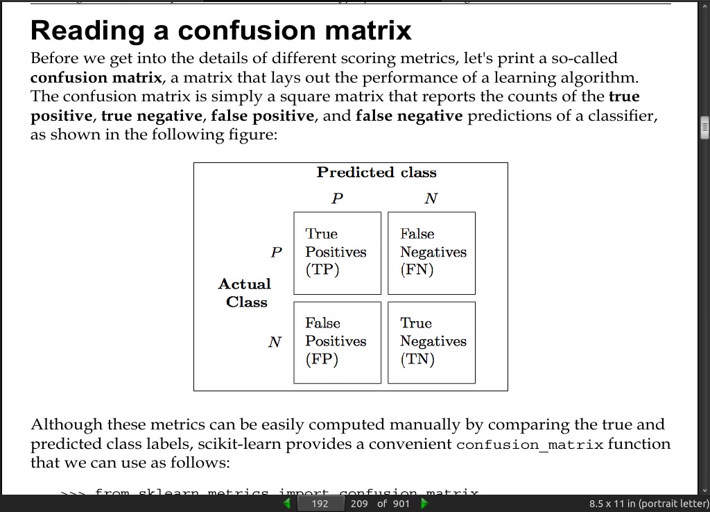
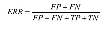
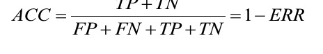
The error (ERR) can be understood as the sum of all false predictions divided by the number of total predictions, and the accuracy (ACC) is calculated as the sum of correct predictions divided by the total number of predictions

page 194:

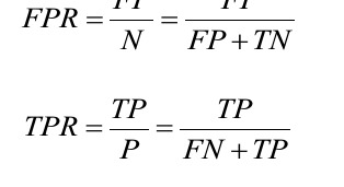
The true positive rate (TPR) and false positive rate (FPR) are performance metrics that are especially useful for imbalanced class problems:

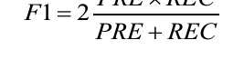
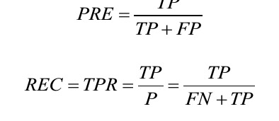
Precision (PRE) and recall (REC) are performance metrics that are related to those true positive and true negative rates, and in fact, recall is synonymous to the true positive rate
In practice, often a combination of precision and recall is used, the so-called F1-score:

page 195:

Remember that the positive class in scikit-learn is the class that is labeled as class 1. If we want to specify a different positive label, we can construct our own scorer via the make_scorer function, which we can then directly provide as an argument to the scoring parameter in GridSearchCV:

>>> from sklearn.metrics import make_scorer, f1_score
>>> scorer = make_scorer(f1_score, pos_label=0)
>>> gs = GridSearchCV(estimator=pipe_svc,
... param_grid=param_grid,
... scoring=scorer,
... cv=10)

Receiver operator characteristic (ROC) graphs are useful tools for selecting models for classification based on their performance with respect to the false positive and true positive rates, which are computed by shifting the decision threshold of the classifier. The diagonal of an ROC graph can be interpreted as random guessing, and classification models that fall below the diagonal are considered as worse than random guessing. A perfect classifier would fall into the top-left corner of the graph with a true positive rate of 1 and a false positive rate of 0. Based on the ROC curve, we can then compute the so-called area under the curve (AUC) to characterize the performance of a classification model
ROC AUC and accuracy metrics mostly agree with each other

page 199:

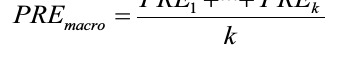
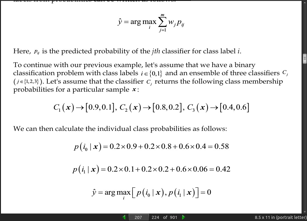
The scoring metrics that we discussed in this section are specific to binary classification systems. However, scikit-learn also implements macro and micro averaging methods to extend those scoring metrics to multiclass problems via One vs. All (OvA) classification. The micro-average is calculated from the individual true positives, true negatives, false positives, and false negatives of the system. For example, the micro-average of the precision score in a k-class system can be calculated as follows:
Micro-averaging is useful if we want to weight each instance or prediction equally, whereas macro-averaging weights all classes equally to evaluate the overall performance of a classifier with regard to the most frequent class labels.

· 07: Combining Different Models for Ensemble Learning

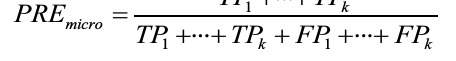
page 202:

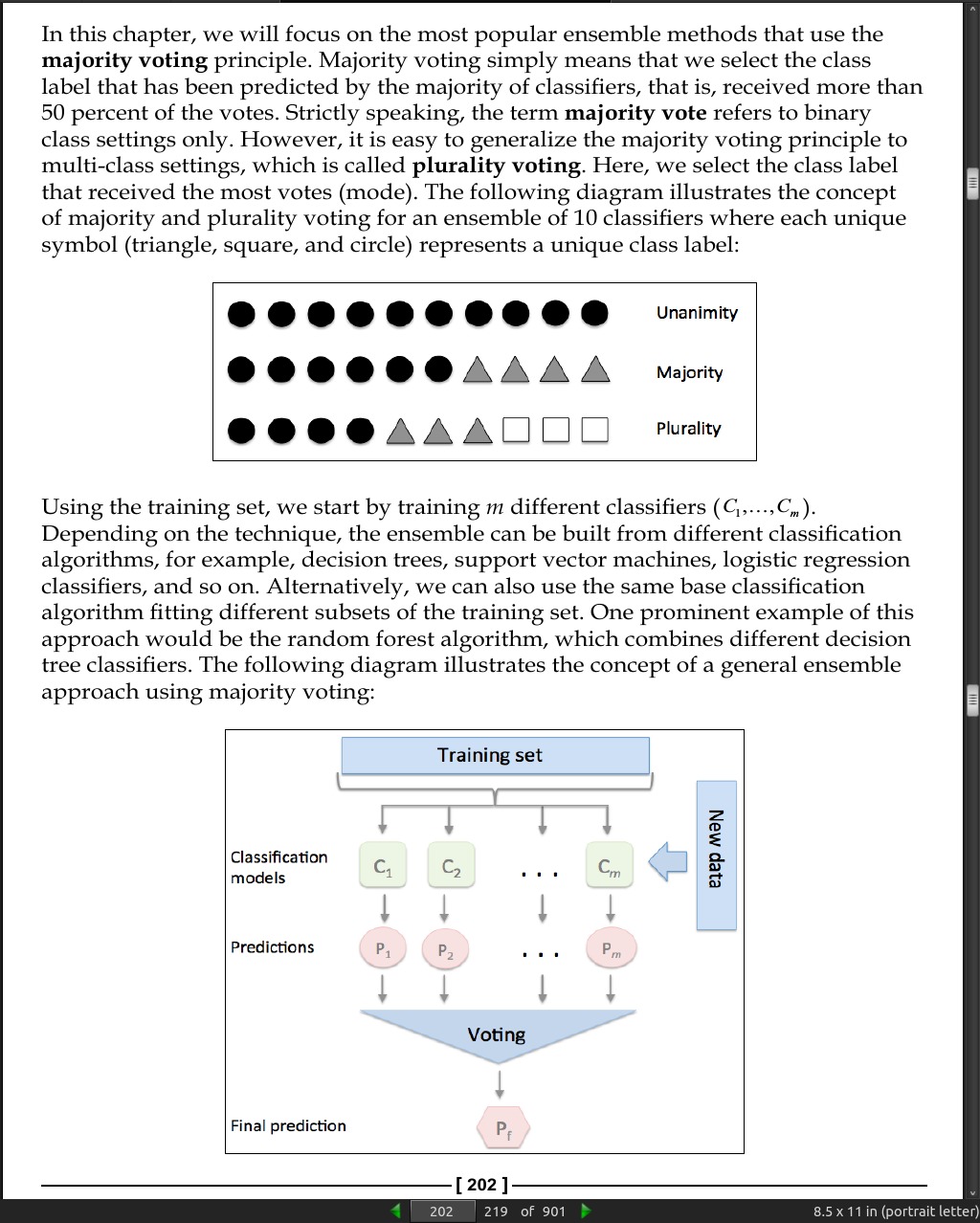
page 203:

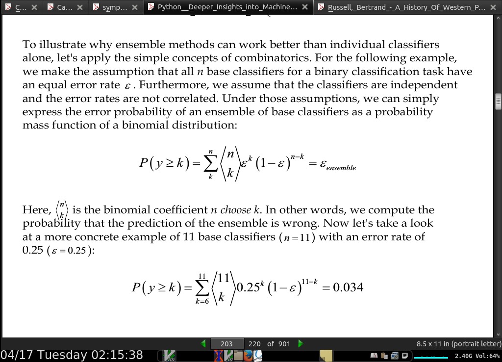
page 207:

page 212:

Although our MajorityVoteClassifier implementation is very useful for demonstration purposes, I also implemented a more sophisticated version of the majority vote classifier in scikit-learn. It will become available as sklearn.ensemble.VotingClassifier in the next release version (v0.17).

page 221:

page 222:

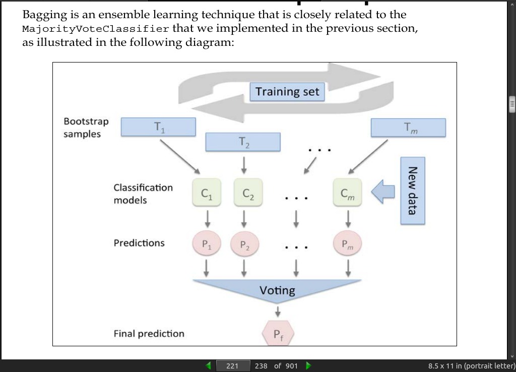
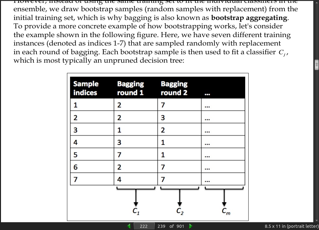
instead of using the same training set to fit the individual classifiers in the ensemble, we draw bootstrap samples (random samples with replacement) from the initial training set, which is why bagging is also known as bootstrap aggregating.
random forests are a special case of bagging where we also use random feature subsets to fit the individual decision trees.

page 226:

The original boosting procedure is summarized in four key steps as follows:

1. Draw a random subset of training samples d1 without replacement from the
training set D to train a weak learner C1.
2. Draw second random training subset d 2 without replacement from the training
set and add 50 percent of the samples that were previously misclassified to
train a weak learner C2.
3.	 Find the training samples d 3 in the training set D on which C 1 and C2
disagree to train a third weak learner C3.
4.	 Combine the weak learners C1 , C2 , and C3 via majority voting.

page 227:

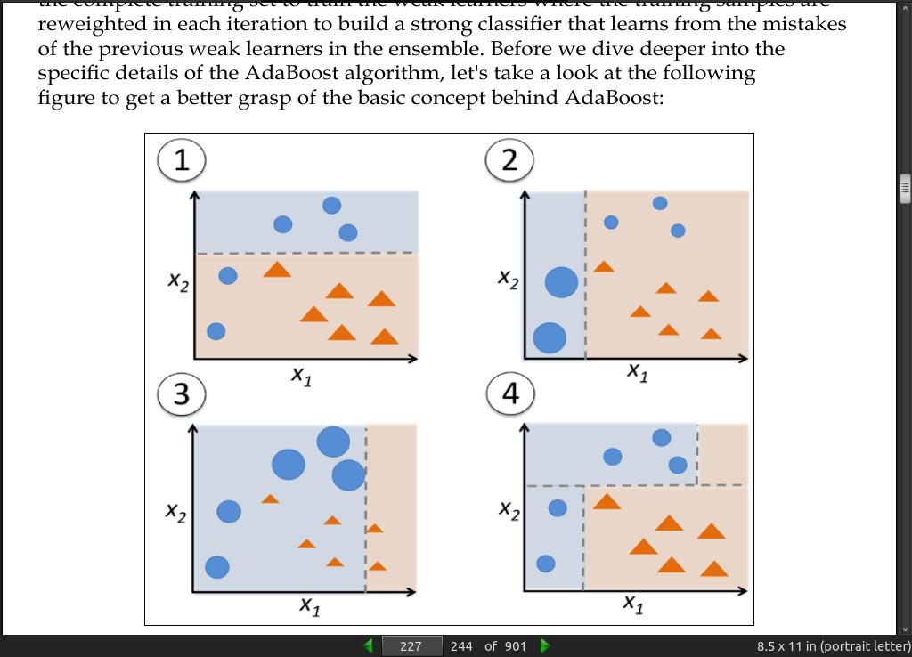
In contrast to the original boosting procedure as described here, AdaBoost uses the complete training set to train the weak learners where the training samples are reweighted in each iteration to build a strong classifier that learns from the mistakes of the previous weak learners in the ensemble.

· 08: Applying Machine Learning to Sentiment Analysis

page 238:

bag-of-words model that allows us to represent text as numerical feature vectors. The idea behind the bag-of-words model is quite simple and can be summarized as follows:

1.	We create a vocabulary of unique tokens—for example, words—from the entire
set of documents.

2.	We construct a feature vector from each document that contains the counts
of how often each word occurs in the particular document.

page 239:

The sequence of items in the bag-of-words model that we just created is also called the 1-gram or unigram model—each item or token in the vocabulary represents a single word. More generally, the contiguous sequences of items in NLP—words, letters, or symbols—is also called an n-gram. The choice of the number n in the n-gram model depends on the particular application; for example, a study by Kanaris et al. revealed that n-grams of size 3 and 4 yield good performances in anti-spam filtering of e-mail messages
raw term frequencies: tf(t,d) — the number of times a term t occurs in a document d.

page 240:

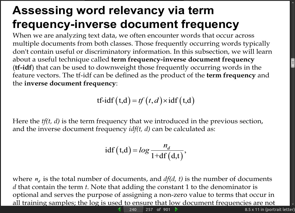
Those frequently occurring words typically don’t contain useful or discriminatory information. In this subsection, we will learn about a useful technique called term frequency-inverse document frequency (tf-idf) that can be used to downweight those frequently occurring words in the feature vectors. The tf-idf can be defined as the product of the term frequency and the inverse document frequency:

page 245:

stop-word removal. Stop-words are simply those words that are extremely common in all sorts of texts and likely bear no (or only little) useful information that can be used to distinguish between different classes of documents. Examples of stop-words are is, and, has, and the like. Removing stop-words can be useful if we are working with raw or normalized term frequencies rather than tf-idfs, which are already downweighting frequently occurring words.

page 249:

we can’t use the CountVectorizer for out-of-core learning since it requires holding the complete vocabulary in memory. Also, the TfidfVectorizer needs to keep the all feature vectors of the training dataset in memory to calculate the inverse document frequencies. However, another useful vectorizer for text processing implemented in scikit-learn is HashingVectorizer.

· 09: Embedding a Machine Learning Model into a Web Application

Flask, SQLite, PythonAnywhere.

· 10: Predicting Continuous Target Variables with Regression Analysis

page 279:

Regression models are used to predict target variables on a continuous scale

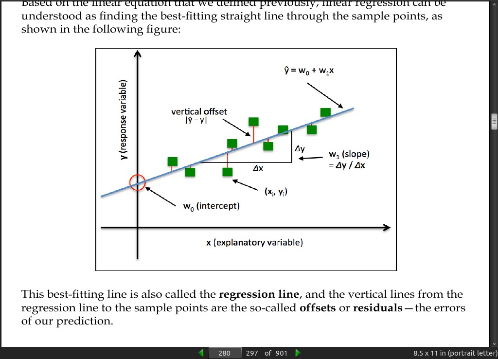
page 280:

This best-fitting line is also called the regression line, and the vertical lines from the regression line to the sample points are the so-called offsets or residuals—the errors of our prediction.

page 287:

Essentially, OLS (Ordinary Least Squares) linear regression can be understood as Adaline without the unit step function so that we obtain continuous target values instead of the class labels -1 and

page 293:

Linear regression models can be heavily impacted by the presence of outliers.
As an alternative to throwing out outliers, we will look at a robust method of regression using the RANdom SAmple Consensus (RANSAC) algorithm, which fits a regression model to a subset of the data, the so-called inliers.
We can summarize the iterative RANSAC algorithm as follows:

1. Select a random number of samples to be inliers and fit the model.

2. Test all other data points against the fitted model and add those points
that fall within a user-given tolerance to the inliers.

3. Refit the model using all inliers.

4. Estimate the error of the fitted model versus the inliers.

5. Terminate the algorithm if the performance meets a certain user-defined
threshold or if a fixed number of iterations has been reached; go back to step
1 otherwise.

page 300:

A Ridge Regression model can be initialized as follows:

>>> from sklearn.linear_model import Ridge
>>> ridge = Ridge(alpha=1.0)

Note that the regularization strength is regulated by the parameter alpha, which is similar to the parameter λ . Likewise, we can initialize a LASSO regressor from the linear_model submodule:

>>> from sklearn.linear_model import Lasso
>>> lasso = Lasso(alpha=1.0)

Lastly, the ElasticNet implementation allows us to vary the L1 to L2 ratio:

>>> from sklearn.linear_model import ElasticNet
>>> lasso = ElasticNet(alpha=1.0, l1_ratio=0.5)

For example, if we set l1_ratio to 1.0, the ElasticNet regressor would be equal to LASSO regression.

page 306:

A random forest, which is an ensemble of multiple decision trees, can be understood as the sum of piecewise linear functions
An advantage of the decision tree algorithm is that it does not require any transformation of the features if we are dealing with nonlinear data.

page 307:

In the context of decision tree regression, the MSE is often also referred to as within-node variance, which is why the splitting criterion is also better known as variance reduction.

· 11: Working with Unlabeled Data – Clustering Analysis

page 314:

Prototype-based clustering means that each cluster is represented by a prototype, which can either be the centroid (average) of similar points with continuous features, or the medoid (the most representative or most frequently occurring point) in the case of categorical features.

page 328:

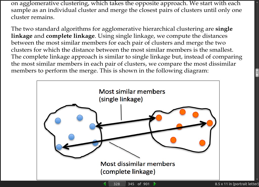
In divisive hierarchical clustering, we start with one cluster that encompasses all our samples, and we iteratively split the cluster into smaller clusters until each cluster only contains one sample. In this section, we will focus on agglomerative clustering, which takes the opposite approach. We start with each sample as an individual cluster and merge the closest pairs of clusters until only one cluster remains.

page 331:

in linkage. However, we should not use the squareform distance matrix that we defined earlier, since it would yield different distance values from those expected. To sum it up, the three possible scenarios are listed here:
Incorrect approach: In this approach, we use the squareform distance matrix. The code is as follows:

>>> from scipy.cluster.hierarchy import linkage
>>> row_clusters = linkage(row_dist,
                           method='complete',
                           metric='euclidean')

Correct approach: In this approach, we use the condensed distance matrix. The code is as follows:

>>> row_clusters = linkage(pdist(df, metric='euclidean'),
                           method='complete')

Correct approach: In this approach, we use the input sample matrix. The code is as follows:

>>> row_clusters = linkage(df.values,
                           method='complete',
                           metric='euclidean')

page 336:

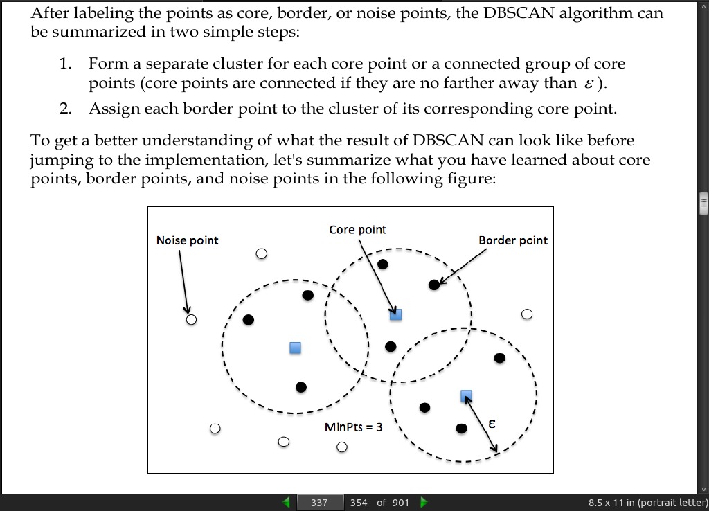
Density-based Spatial Clustering of Applications with Noise (DBSCAN). The notion of density in DBSCAN is defined as the number of points within a specified radius epsilon.

page 337:

· 12: Training Artificial Neural Networks for Image Recognition

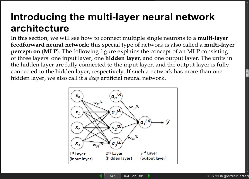
page 347:

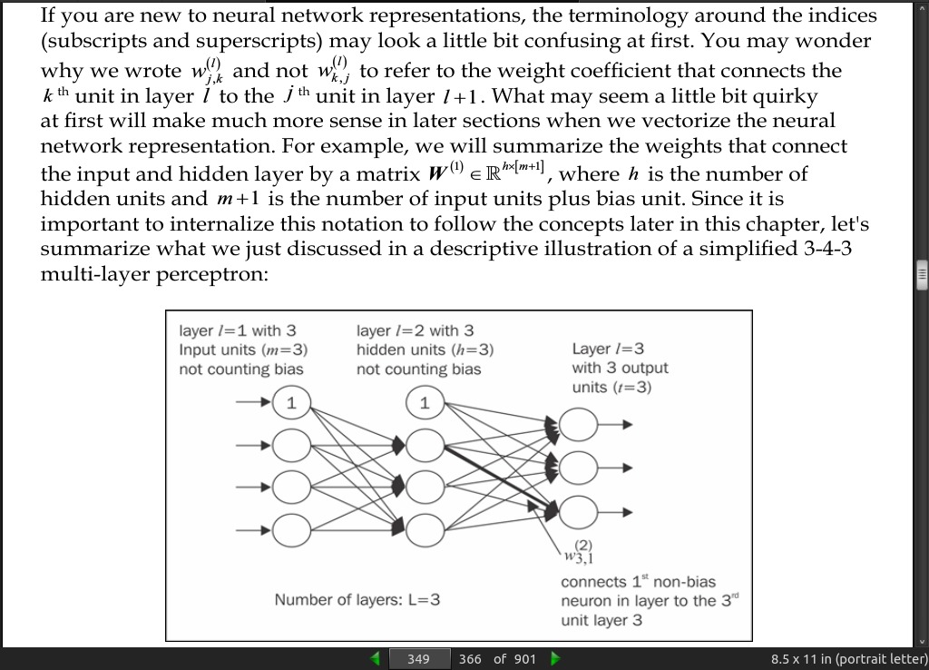
page 349:

page 351:

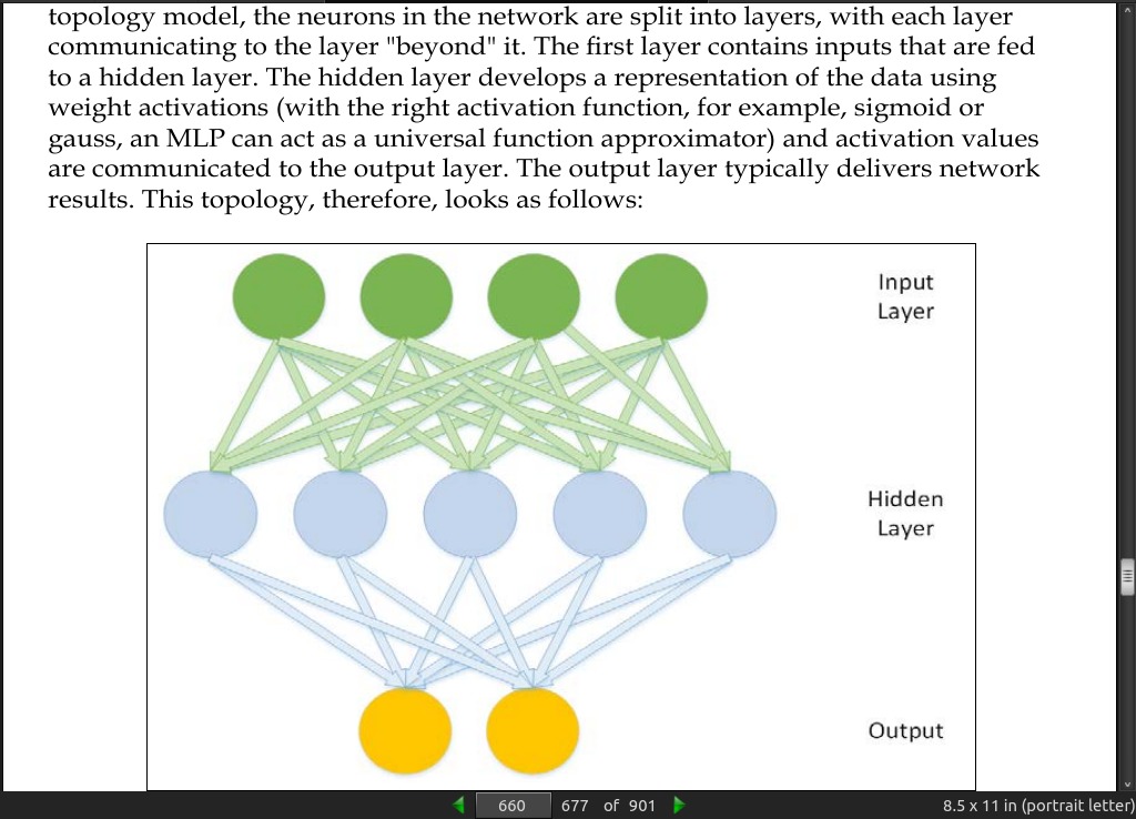
The MLP (Multi-layer perceptron) is a typical example of a feedforward artificial neural network. The term feedforward refers to the fact that each layer serves as the input to the next layer without loops

page 353:

Neural network theory can be quite complex, thus I want to recommend two additional resources that cover some of the concepts that we discuss in this chapter in more detail:
T. Hastie, J. Friedman, and R. Tibshirani. The Elements of Statistical Learning, Volume 2. Springer, 2009.
C. M. Bishop et al. Pattern Recognition and Machine Learning, Volume 1. Springer New York, 2006.

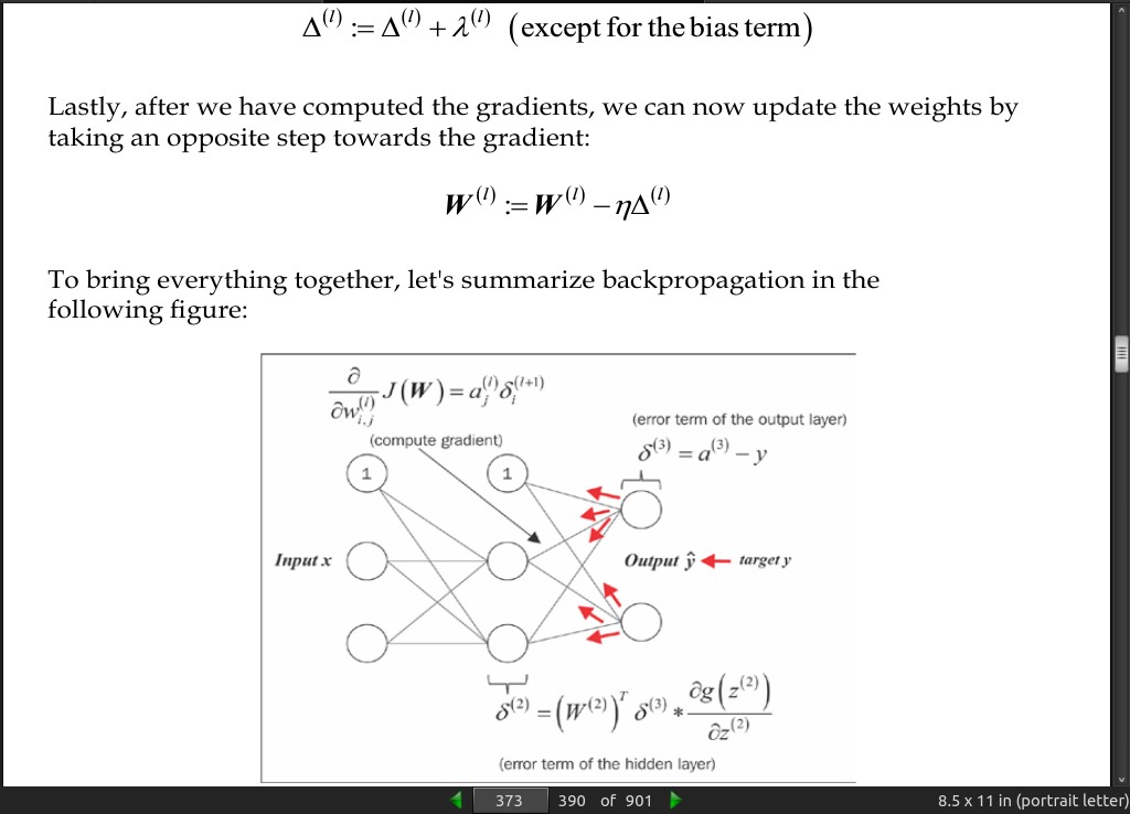
page 373:

page 375:

Automatic differentiation comes with two modes, the forward and the reverse mode, respectively. Backpropagation is simply just a special case of the reverse-mode automatic differentiation. The key point is that applying the chain rule in the forward mode can be quite expensive since we would have to multiply large matrices for each layer (Jacobians) that we eventually multiply by a vector to obtain the output. The trick of the reverse mode is that we start from right to left: we multiply a matrix by a vector, which yields another vector that is multiplied by the next matrix and so on. Matrix-vector multiplication is computationally much cheaper than matrix- matrix multiplication, which is why backpropagation is one of the most popular algorithms used in neural network training.

page 383:

Convolutional Neural Networks (CNNs or ConvNets) gained popularity in computer vision due to their extraordinary good performance on image classification tasks.

page 385:

Recurrent Neural Networks (RNNs) can be thought of as feedforward neural networks with feedback loops or backpropagation through time. In RNNs, the neurons only fire for a limited amount of time before they are (temporarily) deactivated. In turn, these neurons activate other neurons that fire at a later point in time. Basically, we can think of recurrent neural networks as MLPs with an additional time variable.

page 386:

A great collection of Theano tutorials can be found at http://deeplearning.net/ software/theano/tutorial/index.html#tutorial.
There are also a number of interesting libraries that are being actively developed to train neural networks in Theano, which you should keep on your radar:

Pylearn2 (http://deeplearning.net/software/pylearn2/)
Lasagne (https://lasagne.readthedocs.org/en/latest/)
Keras (http://keras.io)

· 13: Parallelizing Neural Network Training with Theano

page 392:

Theano allows you to use GPUs.

page 393:

Tensors can be understood as a generalization of scalars, vectors, matrices, and so on. More concretely, a scalar can be defined as a rank-0 tensor, a vector as a rank-1 tensor, a matrix as rank-2 tensor, and matrices stacked in a third dimension as rank-3 tensors.

page 394:

Configuring Theano.

Can not get Theano to install, Scipy was installed via apt and uninstalling it will also uninstall a number of other programs. So, I skimmed the rest of this chapter. It seems straight forward enough.

page 403:

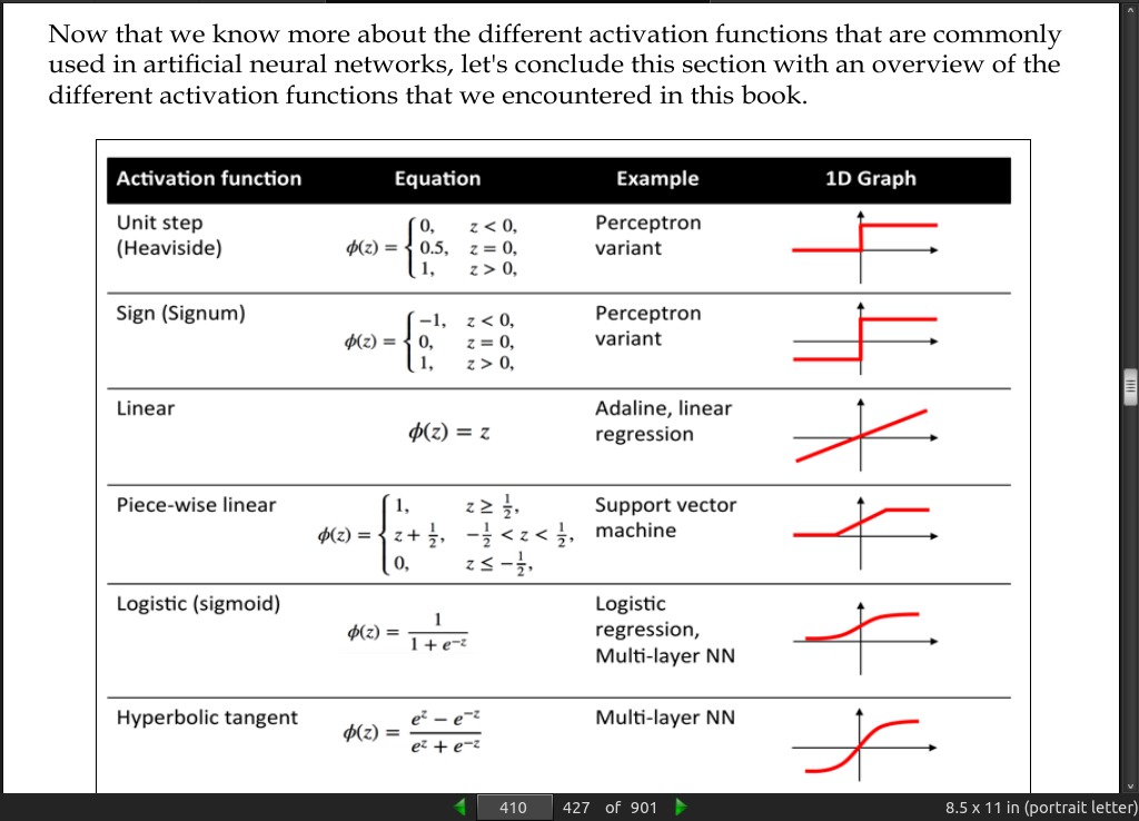
Technically, we could use any function as activation function in multilayer neural networks as long as it is differentiable.

page 404:

page 406:

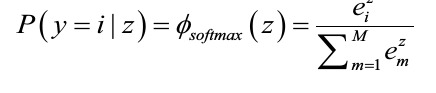
The softmax function is a generalization of the logistic function that allows us to compute meaningful class-probabilities in multi-class settings (multinomial logistic regression).

page 407:

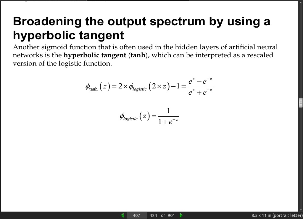
Another sigmoid function that is often used in the hidden layers of artificial neural networks is the hyperbolic tangent (tanh), which can be interpreted as a rescaled version of the logistic function.

page 408:

The advantage of the hyperbolic tangent over the logistic function is that it has a broader output spectrum and ranges the open interval (-1, 1), which can improve the convergence of the back propagation algorithm

page 410:

Keras, built on Theano, skimmed, looks straight forward.

page 415:

Although Keras is a great library for implementing and experimenting with neural networks, there are many other Theano wrapper libraries that are worth mentioning. A prominent example is Pylearn2 (http://deeplearning.net/software/ pylearn2/), which has been developed in the LISA lab in Montreal. Also, Lasagne (https://github.com/Lasagne/Lasagne) may be of interest to you if you prefer a more minimalistic but extensible library, that offers more control over the underlying Theano code.

page 417:

follow the works of the leading experts in this field, such as Geoff Hinton (http://www.cs.toronto.edu/~hinton/), Andrew Ng (http://www.andrewng. org), Yann LeCun (http://yann.lecun.com), Juergen Schmidhuber (http:// people.idsia.ch/~juergen/), and Yoshua Bengio (http://www.iro.umontreal. ca/~bengioy),

· 01: Thinking in Machine Learning

page 424:

This [The expression of emotion in 20th century books (Acerbi et al, 2013)] study is interesting for several reasons. Firstly, it is an example of data-driven science, where previously considered soft sciences, such as sociology and anthropology, are given a solid empirical footing.

page 429:

page 446:

page 448:

//UML, Unified Modeling Language.

page 451:

//State diagrams.

· 02: Tools and Techniques

page 458:

NumPy builds on these data objects by providing two further objects: an N-dimensional array object (ndarray) and a universal function object (ufunc). The ufunc object provides element-by-element operations on ndarray objects, allowing typecasting and array broadcasting. Typecasting is the process of changing one data type into another, and broadcasting describes how arrays of different sizes are treated during arithmetic operations.

page 475:

There are two different K-NN classifiers in Sklearn. KNeighborsClassifier requires the user to specify k, the number of nearest neighbors. RadiusNeighborsClassifier, on the other hand, implements learning based on the number of neighbors within a fixed radius, r, of each training point.

page 477:

For the Ordinary Least Squares to work, we assume that the features are independent. When these terms are correlated, then the matrix, X, can approach singularity. This means that the estimates become highly sensitive to small changes in the input data. This is known as multicollinearity and results in a large variance and ultimately instability.

page 478:

Ridge regression not only addresses the issue of multicollinearity, but also situations where the number of input variables greatly exceeds the number of samples. The linear_model.Ridge() object uses what is known as L2 regularization. Intuitively, we can understand this as adding a penalty on the extreme values of the weight vector. This is sometimes called shrinkage because it makes the average weights smaller. This tends to make the model more stable because it reduces its sensitivity to extreme values.
The Sklearn object, linear_model.ridge, adds a regularization parameter, alpha. Generally, small positive values for alpha improves the model’s stability. It can either be a float or an array. If it is an array, it is assumed that the array corresponds to specific targets, and therefore, it must be the same size as the target.
Determining what is redundant or irrelevant is the major function of dimensionality reduction algorithms. There are basically two approaches: feature extraction and feature selection. Feature selection attempts to find a subset of the original feature variables. Feature extraction, on the other hand, creates new feature variables by combining correlated variables.

page 479:

most common feature extraction algorithm, that is, Principle Component Analysis or PCA. This uses an orthogonal transformation to convert a set of correlated variables into a set of uncorrelated variables. The important information, the length of vectors, and the angle between them does not change.
Probably the most versatile kernel function, and the one that gives good results in most situations, is the Radial Basis Function (RBF). The rbf kernel takes a parameter, gamma, which can be loosely interpreted as the inverse of the sphere of influence of each sample. A low value of gamma means that each sample has a large radius of influence on samples selected by the model. The KernalPCA fit_transform method takes the training vector, fits it to the model, and then transforms it into its principle components.

· 03: Turning Data into Information

page 483:

For data to become information, it requires some meaningful structure.

page 484:

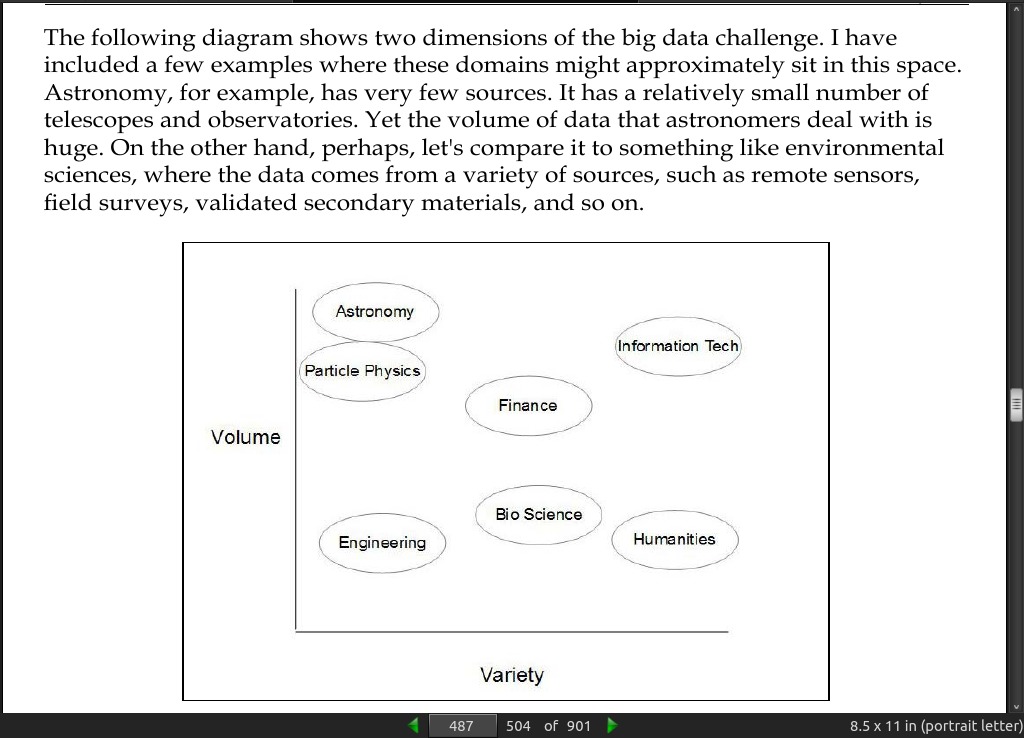
When faced with an unseen dataset, the first phase is exploration. Data exploration involves examining the components and structure of data. How many samples does it contain, and how many dimensions are in each sample? What are the data types of each dimension? We should also get a feel for the relationships between variables and how they are distributed. We need to check whether the data values are in line with what we expect. Are there are any obvious errors or gaps in the data?

page 485:

Parallelism is a growing area of machine learning, and it encompasses a number of different approaches, from harnessing the capabilities of multi-core processors, to large-scale distributed computing on many different platforms. Probably, the most common method is to simply run the same algorithm on many machines, each with a different set of parameters. Another method is to decompose a learning algorithm into an adaptive sequence of queries, and have these queries processed in parallel. A common implementation of this technique is known as MapReduce, or its open source version, Hadoop.

page 487:

Integrating different data sets can take a significant amount of development time; up to 90 percent in some cases.

page 489:

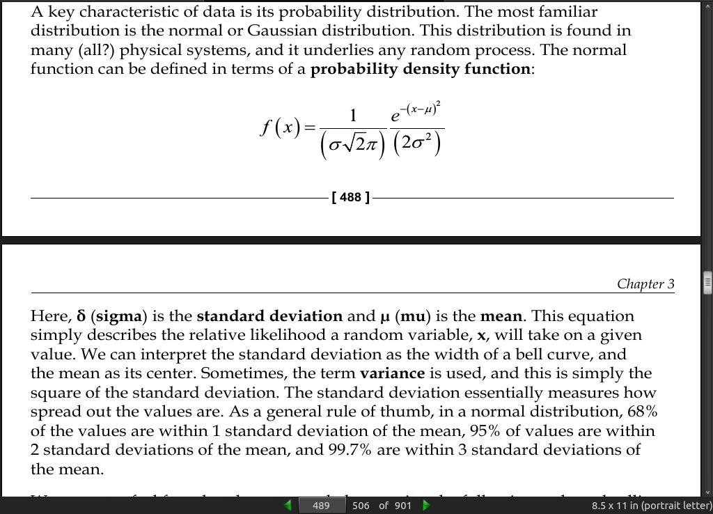
page 490:

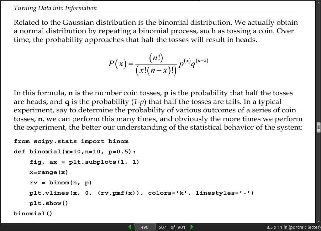
page 491:

page 492:

page 501:

page 503:

Another format that we are likely to come across is the Acrobats Portable Document Format (PDF). Importing data from PDF files can be quite difficult because PDF files are built on page layout primitives, and unlike HTML or JSON, they do not have meaningful markup tags. There are several non-Python tools for turning PDFs into text such as pdftotext. This is a command line tool that is included in many Linux distributions and is also available for Windows. Once we have converted the PDF file into text, we still need to extract the data, and the data embedded in the document determines how we can extract it. If the data is separated from the rest of the document, say in a table, then we can use Python’s text parsing tools to extract it. Alternatively, we can use a Python library for working with PDF documents such as pdfminer3k.

· 04: Models – Learning from Information

· 05: Linear Models

page 529:

This is described by the terms variance (for over fitting models) and bias (for under fitting models). A linear model is typically low-variance and high-bias.

page 536:

The normal equation:

w = (X^T X)^-1 * X^T y

can be used instead of gradient descent.

page 538:

One of the advantages of using the normal equation is that you do not need to worry about feature scaling.
Another advantage of the normal equation is that you do not need to choose the learning rate.
The normal equation has its own particular disadvantages; foremost is that it does not scale as well when we have data with a large number of features. We need to calculate the inverse of the transpose of our feature matrix, X. This calculation results in an n by n matrix. Remember that n is the number of features. This actually means that on most platforms the time it takes to invert a matrix grows, approximately, as a cube of n. So, for data with a large number of features, say greater than 10,000, you should probably consider using gradient descent rather than the normal equation. Another problem that arises when using the normal equation is that, when we have more features than training data, that is, when n is greater than m, the normal equation without regularization will not work. This is because the matrix, XTX, is non-transposable, and so there is no way to calculate our term, (XTX)^-1.

page 544:

In the one versus all approach, [to multiclass classification] a single multiclass problem is transformed into a number of binary classification problems. This is called the one versus all technique because we take each class in turn and fit a hypothesis function for that particular class, assigning a negative class to the other classes. We end up with different classifiers, each of which is trained to recognize one of the classes.
With another approach called the one versus one method, a classifier is constructed for each pair of classes. When the model makes a prediction, the class that receives the most votes wins.
Sklearn implements the one versus all algorithm using the OneVsRestClassifier /span> class and the one versus one algorithm with OneVsOneClassifier.

page 545:

We mentioned earlier that linear regression can become unstable, that is, highly sensitive to small changes in the training data, if features are correlated. Consider the extreme case where two features are perfectly negatively correlated such that any increase in one feature is accompanied by an equivalent decrease in another feature. When we apply our linear regression algorithm to just these two features, it will result in a function that is constant, so this is not really telling us anything about the data. Alternatively, if the features are positively correlated, small changes in them will be amplified. Regularization helps moderate this.

page 546:

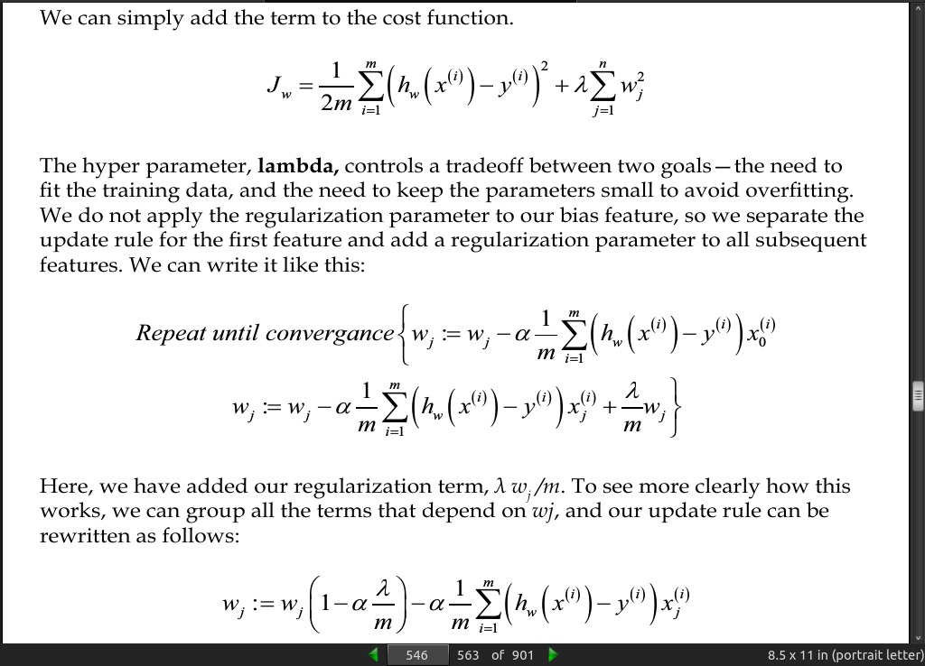
page 547:

Ridge regression is sometimes referred to as using the L2 norm, and lasso regularization, the L1 norm.

· 06: Neural Networks

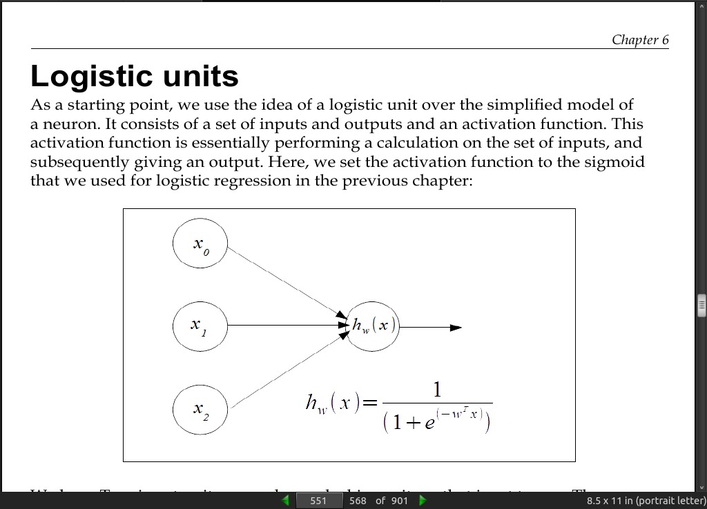
page 549:

Nice chapter, describes the algorithms well.

page 551:

· 07: Features – How Algorithms See the World

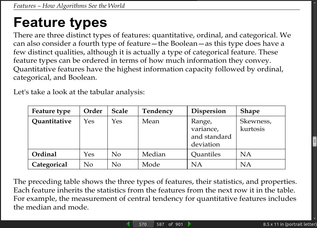
page 569:

The right features, sometimes called attributes, are the central component for machine learning models. A sophisticated model with the wrong features is worthless.

page 570:

page 582:

fill in the missing values through a process of imputation. For classification, we can simply use the statistics of the mean, median, and mode over the observed features to impute the missing values.

Many machine learning algorithms require that features are standardized. This means that they will work best when the individual features look more or less like normally distributed data with near-zero mean and unit variance. The easiest way to do this is by subtracting the mean value from each feature and scaling it by dividing by the standard deviation. This can be achieved by the scale() function or the standardScaler() function in the sklearn.preprocessing() function. Although these functions will accept sparse data, they probably should not be used in such situations because centering sparse data would likely destroy its structure. It is recommended to use the MacAbsScaler() or maxabs_scale() function in these cases. The former scales and translates each feature individually by its maximum absolute value. The latter scales each feature individually to a range of [-1,1]. Another specific case is when we have outliers in the data. In these cases using the robust_scale() or RobustScaler() function is recommended.

· 08: Learning with Ensembles

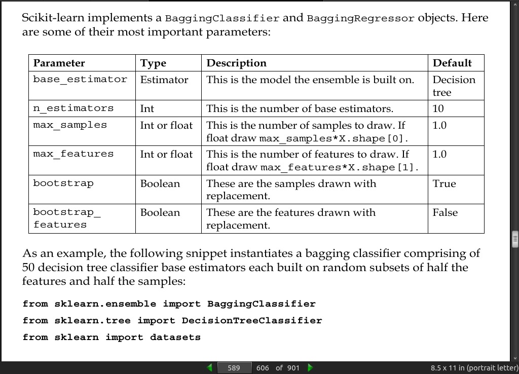
page 589:

Tree-based models are particularly well suited to ensembles, primarily because they can be sensitive to changes in the training data.
builds each tree using a different random subset of the features and is therefore called a random forest.

page 601:

Generally, in classification tasks, there are three reasons why a model may misclassify a test instance. Firstly, it may simply be unavoidable if features from different classes are described by the same feature vectors. In probabilistic models, this happens when the class distributions overlap so that an instance has non-zero likelihoods for several classes. Here we can only approximate a target hypothesis.
The second reason for classification errors is that the model does not have the expressive capabilities to fully represent the target hypothesis. For example, even the best linear classifier will misclassify instances if the data is not linearly separable. This is due to the bias of the classifier. Although there is no single agreed way to measure bias, we can see that a nonlinear decision boundary will have less bias than a linear one, or that more complex decision boundaries will have less bias than simpler ones. We can also see that tree models have the least bias because they can continue to branch until only a single instance is covered by each leaf.

page 602:

Now, it may seem that we should attempt to minimize bias; however, in most cases, lowering the bias tends to increase the variance and vice versa. Variance, as you have probably guessed, is the third source of classification errors. High variance models are highly dependent on training data. The nearest neighbor’s classifier, for example, segments the instance space into single training points. If a training point near the decision boundary is moved, then that boundary will change. Tree models are also high variance, but for a different reason. Consider that we change the training data in such a way that a different feature is selected at the root of the tree. This will likely result in the rest of the tree being different.

Bagging is primarily a variance reduction technique and boosting is primarily a bias reduction technique.
Bagging ensembles work most effectively with high variance models, such as complex trees, whereas boosting is typically used with high bias models such as linear classifiers.

· 09: Design Strategies and Case Studies

page 605:

The importance of defining a scoring strategy should not be underestimated, and in Sklearn, there are basically three approaches:
Estimator score: This refers to using the estimator’s inbuilt score() method, specific to each estimator
Scoring parameters: This refers to cross-validation tools relying on an internal scoring strategy
Metric functions: These are implemented in the metrics module

page 606:

A better way to measure performance is using by precision, (P) and Recall, (R). If you remember from the table in Chapter 4, Models – Learning from Information, precision, or specificity, is the proportion of predicted positive instances that are correct, that is, TP/(TP+FP). Recall, or sensitivity, is TP/(TP+FN). The F-measure is defined as 2RP/ (R+P). These measures ignore the true negative rate, and so they are not making an evaluation on how well a model handles negative cases.

page 612:

Grid search is probably the most used method of optimization hyper parameters, however, there are times when it may not be the best choice. The RandomizedSearchCV object implements a randomized search over possible parameters. It uses a dictionary similar to the GridSearchCV object, however, for each parameter, a distribution can be set, over which a random search of values will be made. If the dictionary contains a list of values, then these will be sampled uniformly. Additionally, the RandomizedSearchCV object also contains an n_iter parameter that is effectively a computational budget of the number of parameter settings sampled. It defaults to 10, and at high values, will generally give better results. However, this is at the expense of runtime.
There are alternatives to the brute force approach of the grid search, and these are provided in estimators such as LassoCV and ElasticNetCV. Here, the estimator itself optimizes its regularization parameter by fitting it along a regularization, path. This is usually more efficient than using a grid search.

Module 3: Advanced Machine Learning with Python

· 01: Unsupervised Machine Learning

page 631:

Unsupervised learning techniques are a valuable set of tools for exploratory analysis.

page 634:

In summary, the covariance matrix is used to calculate Eigenvectors. An orthonormalization process is undertaken that produces orthogonal, normalized vectors from the Eigenvectors. The eigenvector with the greatest eigenvalue is the first principal component with successive components having smaller eigenvalues. In this way, the PCA [Principle Component Analysis] algorithm has the effect of taking a dataset and transforming it into a new, lower-dimensional coordinate system.

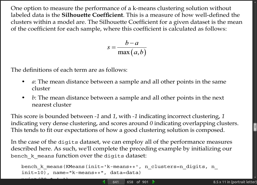
page 641:

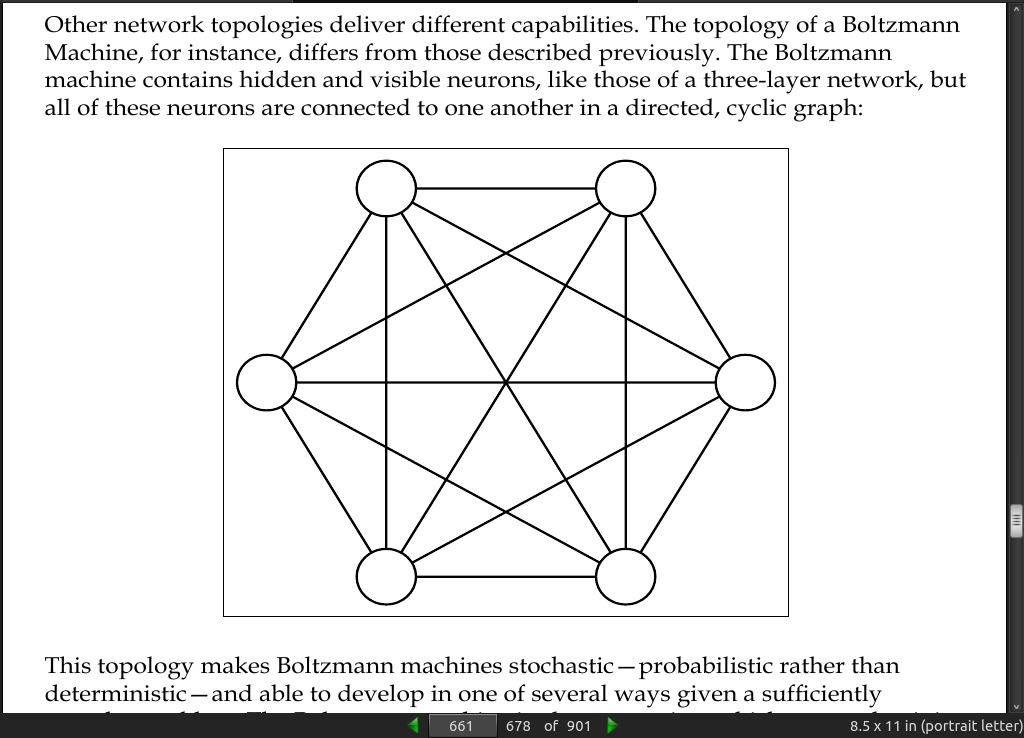
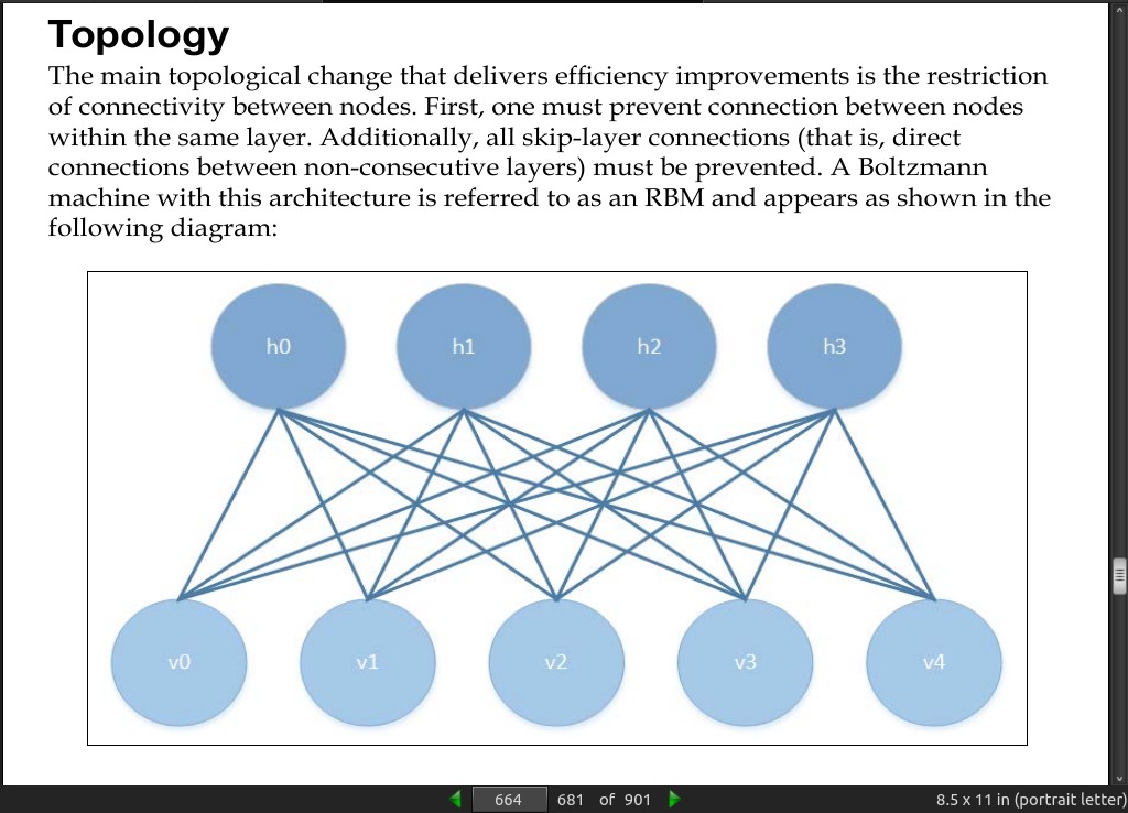
· 02: Deep Belief Networks

page 658:

The RBM [Restricted Boltzmann Machine] is a form of recurrent neural network.

page 660:

page 661:

This topology makes Boltzmann machines stochastic—probabilistic rather than deterministic
[RBM] is an energy-based model, which means that it uses an energy function to associate an energy value with each configuration of the network.

page 664:

page 679:

The RBM is most commonly used as a pretraining mechanism for a highly effective deep network architecture called a DBN [deep belief networks]. DBNs are extremely powerful tools to learn and classify a range of image datasets. They possess a very good ability to generalize to unknown cases and are among the best image-learning tools available.
it has been noted that even if the layers don’t contain very many nodes, with enough layers, more or less any function can be modeled.

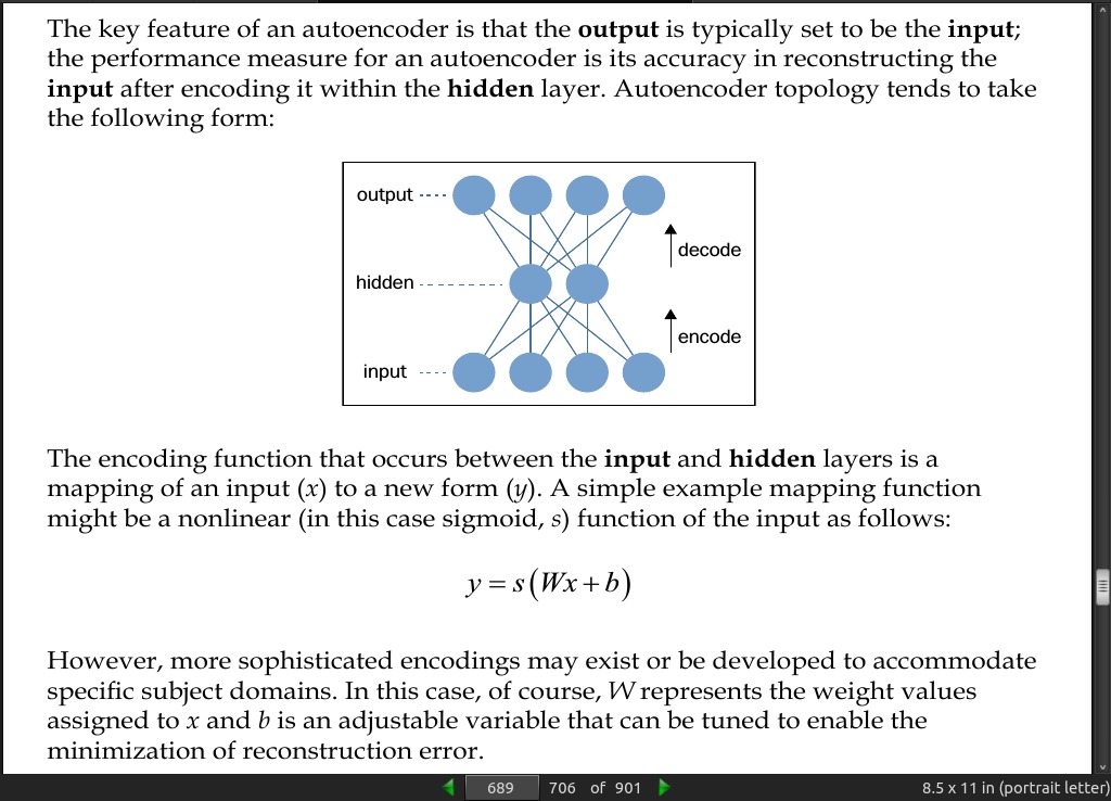
· 03: Stacked Denoising Autoencoders

page 688:

An autoencoder is a simple three-layer neural network whose output units are directly connected back to the input units. The objective of the autoencoder is to encode the i-dimensional input into an h-dimensional representation, where h < i, before reconstructing (decoding) the input at the output layer. The training process involves iteration over this process until the reconstruction error is minimized

page 689:

page 691;

a denoising autoencoder can work effectively with minimal preprocessing.

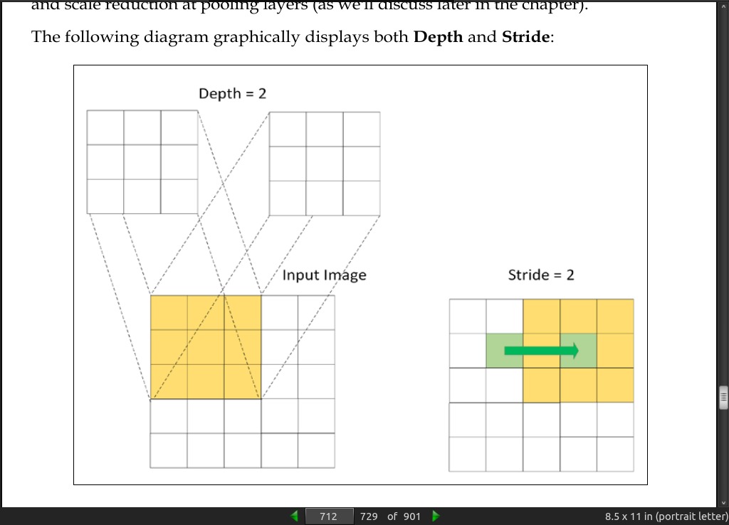
· 04: Convolutional Neural Networks

page 708:

The design of convolutional neural networks takes inspiration from the visual cortex
Google’s DeepDream program, which became well-known for its overtrained, hallucinogenic imagery, also uses a convolutional neural network.
Facebook uses convolutional nets in face verification (DeepFace).

page 709:

Perhaps the most immediate difference between a convolutional neural network and most other networks is that all of the neurons in a convnet are identical! All neurons possess the same parameters and weight values. As you can see, this will immediately reduce the number of parameter values controlled by the network, bringing substantial efficiency savings. It also typically improves network learning rate as there are fewer free parameters to be managed and computed over.

page 712:

page 720:

GoogLeNet was designed to tackle computer vision challenges involving Internet-quality image data, that is, images that have been captured in real contexts where the pose, lighting, occlusion, and clutter of images vary significantly. GoogLeNet was applied to the 2014 ImageNet challenge with noteworthy success, achieving only 6.7% error rate on the test dataset. ImageNet images are small, high-granularity images taken from many, varied classes.

· 05: Semi-Supervised Learning

· 06: Text Feature Engineering

page 759:

“The features you use influence more than everything else the result. No algorithm alone, to my knowledge, can supplement the information gain given by correct feature engineering.” -(Luca Massaron)

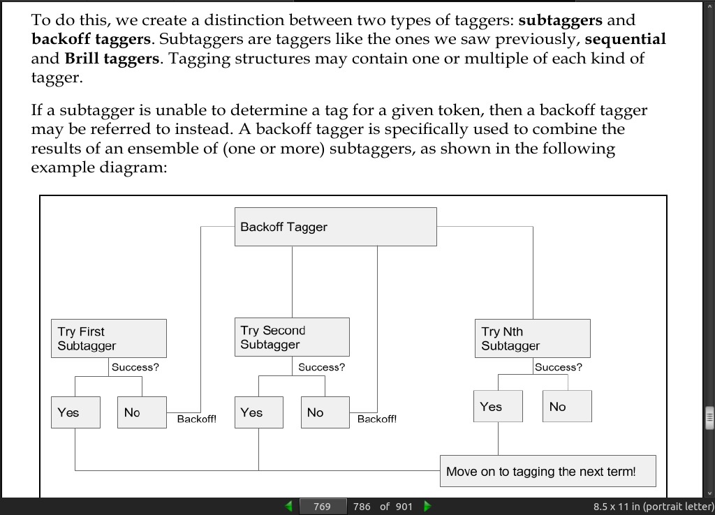
page 769:

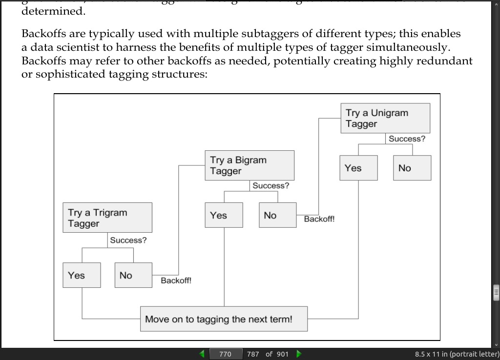
page 770:

· 07: Feature Engineering Part II

page 798:

there is a specific multicollinearity test that’s worth considering; namely, inspecting the eigenvalues of our data’s correlation matrix.

page 805:

Deep learning algorithms tend to perform better on less-engineered data than shallower models and it might be that less work is needed to improve results.

· 08: Ensemble Methods

page 862:

typical goal in applied machine learning contexts is to reduce the factor of training time to data change frequency to the smallest value possible.

· 09: Additional Python Machine Learning Tools

page 866:

Lasagne was created, to call Theano functions and return Theano expressions or numpy data types, in a much less complex and more easily understood manner than the same operations written in native Theano code.

page 869:

TensorFlow

Home · Book Reports · 2018 · Python - Deeper Insights Into Machine Learning

Thoughts

Other

Links

Code Examples

Further Reading

Exceptional Excerpts

Table of Contents

Module 1: Python Machine Learning

Module 2: Designing Machine Learning Systems with Python

Module 3: Advanced Machine Learning with Python

Module 1: Python Machine Learning

· 01: Giving Computers the Ability to Learn from Data

page 004:

page 010:

page 012:

page 14:

· 02: Training Machine Learning Algorithms for Classification

page 24:

page 25:

page 026:

page 035:

page 36:

page 44:

page 45:

· 03: A Tour of Machine Learning Classifiers Using Scikit-learn

page 51:

page 52:

page 55:

page 60:

page 61:

page 68:

page 70:

page 71:

page 074:

page 76:

page 078:

page 79:

page 84:

page 85:

page 86:

page 94:

page 95:

page 96:

page 98:

· 04: Building Good Training Sets – Data Preprocessing

page 103:

page 104:

page 105:

page 106:

page 112:

page 113:

page 120:

page 128:

· 05: Compressing Data via Dimensionality Reduction

page 130:

page 131:

page 133:

page 140:

page 141:

page 151:

page 153:

page 154:

page 169:

· 06: Learning Best Practices for Model Evaluation and Hyperparameter Tuning

page 174:

page 176:

page 177:

page 178:

page 179:

page 182:

page 183:

page 187:

page 188:

page 189:

page 190:

page 192:

page 193:

page 194:

page 195: